Lecture 06
Reading material: Section 3.1 - 3.3 of CSSB.
Recap & Intro
Last time, we discussed correlations, the concept of orthogonality, inner products, the issue with correlations and the use of averaging to filter out noise.
In this lecture and the next we will try to tie together a few concepts introduced so far to understand the Fourier series and expansions.
Some background
We tend to think of a vector as a tuple or collection of real numbers. Intuitively, this makes sense to us because in two and three dimensions these correspond to the familiar coordinates from 2D and 3D geometry. Vector addition, multiplication etc. are thus intuitively familiar to us and we have no qualms with writing: let refer to a vector in 3D. In fact, we are even comfortable with: let . Now let us take a step back and think of .
What is it?
Vector spaces
We naturally think of as the space in which or or our vectors live in or belong to - a vector space. How is this formalized? Well, recall from BIOE210[1] that we have field axioms that specify the rules followed by elements that we can do algebra with. Similarly, there are axioms or rules that a space must satisfy to be a vector space. Note that there is no specification in the field axioms on what the elements and are: only that they follow some rules.
In the same vein, there are no restrictions on what we can consider as vectors in a vector space as long as they follow these rules. Don't be intimidated by the math on that page: you already know a few vector spaces! For example and are all vector spaces which follow those rules; only that the rules are written up in an abstract way.
Basis
Now follows a slightly wordy definition:
Take note of how we have written a summation to express in terms of the basis. This way of writing vectors will show up a lot.
Whenever we talked of vectors, we have been implicitly using a basis – in fact the standard basis which are defined as vectors that are zero in all entries except the -th one. Thus even a vector like is actually where
As mentioned above, the choice of the basis vector set is not unique. It just so happens that the set as the basis for is extremely convenient. The construction below shows how the same point in can be represented in two different bases.
The black axes obviously represent the standard basis and . The blue pair of rays represent the directions given by a new set of basis vectors (in black) that you can choose by entering the vectors and into the input boxes. Since we are in 2D or equivalently , we need a pair of basis vectors and each vector has two entries, and .
Then moving the blue point around shows how it is represented in coordinates that utilize the usual basis (in black) and the newly chosen basis (in blue). Thus the blue coordinates & the black coordinates represent the same vector in but with different sets as the basis.
This non-uniqueness of the basis set is not a peculiar feature of just or .
As shown above has the familiar basis that we are used to seeing. But we can also find another basis set. For example consider the polynomials in given by
One can show that the set is also a basis for .
Be sure to work this out: Verify (a) the application of the defining equation to write out the basis vectors as well as (b) the fact that is indeed in this basis.
Why do we care?
Apart from providing a preview of what will be a major & crucial topic in any course on linear algebra[2]; the main takeaway here is that representing a problem or situation in a different basis can often make things simpler or provide more insight into a problem. For example polar & spherical coordinates often simplify problems in physics as you may recall.
Indeed, many important techniques you will learn, including Principal Components Analysis, Singular Value Decomposition, eigendecompositions etc. are all essentially a change of basis to some particularly useful basis vectors. Moreover, change of basis calculations form an extremely important part of various analytical & problem solving techniques including solving differential equations, implementing matrix multiplications, etc.
More pertinently for us, recall that we can think of signals and functions as being elements of certain vector space. It turns out that the in the continuous domain, what is akin to the change-of-basis we discussed above are called integral transforms but more on that later.
Fourier Transform(s)
CSSB talks about four different "transforms" in the forward and reverse directions[3]. They are listed as:
| Transform name | Applicabiliy | Acronynm | Implementation/Usage |
|---|---|---|---|
| Discrete Fourier Transform | applicable to periodic discrete signals | DFT | all real world applications |
| Fourier Series | applicable to periodic and continuous signals | FS | analytical computations |
| Fourier Transform | applicable to aperiodic and continuous signals | FT | analytical computations |
| Discrete Time Fourier Transform | theoretically applicable to aperiodic & discrete signals | DTFT | not possible |
Please take care to use the right name because each of the techniques have slightly different areas of applicability as listed in the table. In the words of one bestselling author:
You might be thinking that the names given to these four types of Fourier transforms are confusing and poorly organized. You're right; the names have evolved rather haphazardly over 200 years. There is nothing you can do but memorize them and move on.
~ S. W. Smith
We will start with the DFT above, and discuss each in turn, though we may not follow the unwieldy notation used in CSSB. We start with the DFT because it is directly related to the discussions we have had above.
Discrete Fourier Transform (DFT)
Given one period of discrete periodic signal as vector of length we define the DFT of it as the sequence of complex numbers given by:
Note the similarity of the above summation with those we have been using to express vectors in terms of different basis. This is no coincidence because the inverse DFT is:
We finally hit pay dirt for mining through all the math so far.
One naturally wonders why we would bother to write a signal in terms of complex exponentials. Here is where we tie up another thread we introduced a couple of lectures back via Euler's formula: complex exponentials are sinusoids!
Thus in the above:
One should think of this as evaluating a sine and cosine of frequency at the time .
Note that the summation is over in (3): Therefore, we are expressing the original signals as a summation of sinusoids of different frequencies! This is useful because sinusoids are the "nicest" periodic functions in a sense[4].
Recall from Lecture 03 that a general sinusoid can be written in terms of pure sines & cosines without phases. Therefore, rather than having to find the coefficient for the sine part and the coefficient for the cosine part separately (as we will in next lecture), the complex formulation above does it in one shot.
We have used square brackets in the above in the usual sense for discrete signals but also pay close attention to the use of vs (one refers to the signal and the other its transform).
The normalization factor we have used above is ; which lends credence to our interpretation as a change of basis. CSSB and most other texts/implementations present an unnormalized DFT and normalized iDFT (by ); it changes things very little as long as one is consistent.
Fourier's great insight was that theoretically, any periodic function can be expressed in terms of a summation of sines & cosines a constant. In practice though, there are a few caveats. For example, the function to be expressed needs to be "nice" in certain mathematical terms. Sometimes the summation needed might be an infinite one which we cannot do on a computer. The demonstration below illustrates this with a square wave. The first collection of plots (of different colors) show the sinusoids of five different frequencies being added together to create the plot immediately below it (green). The green plot can be changed by using the checkboxes to add/remove sine wave of a particular frequency. The last plot (brown) shows what happens when you increase the number of frequencies being summed together (using the slider). At its maximum value, we see that we get a very good approximation of a square wave.
In the above definition we took a complete period of a signal when we computed its transform. This is an implicit assumption whenever we perform the DFT. In practice, it is rarely the case that we will have one complete period of the signal we are performing DFT on which leads to some artifacts . These will be the subject of subsequent lectures.
Note that while we discuss other flavors of the transform next; the only one we can implement and perform on real world signals is the DFT via a computer. Nevertheless, the other transforms are important to know for purposes of analysis and problem solving and we look at these next.
To show they are inverses one should go back and forth between equations – put (2) in (3) and get the identity & vice versa. However, the ideas are essentially the same so it suffices to just do one. To start, note that in (2) the is a dummy variable used only for summation and is distinct from the in (3) where is referring to the -th coordinate of . So start by rewriting the forward transform as:
Finally show that the leftover sum therefore is simply since the only nonzero term arises when .
Fourier Series
In the above discussion, we had a discrete periodic signal to begin with. What happens if instead we have a continuous periodic signal? We no longer have any indices to sum over; so we should adjust our equations a bit. While in terms of implementation, everything in a computer relies on the DFT, conceptually we tend to think in terms of continuous signals and so this is a practical concern.
To go from discrete to continuous recall that we summed over a complete period of a signal. For continuous signals the summation becomes an integration and just like before we integrate over a full period . Next, the summation variable turns into the integration variable . Moreover as we replace we also do:
Thus we get that Fourier Series corresponding to a periodic signal over one period is given as:
where we have normalized by the period . The quantity should be familiar to us from our discussion of periodic signals and is in the context of Fourier analysis called the fundamental frequency. Moreover, in literature it is common to call (4) and (2) as forward or analysis equations and the inverse transform as in (3) as the synthesis equation because these synthesize our signal out of sinusoids. Thus, for a continuous periodic signal, the synthesis equation is given by:
Note that the synthesis equation is still a summation and the analysis equations generates an infinite sequence of Fourier coefficients . This explains the reason why we call it the Fourier Series. Ideally, we should have called the DFT the Discrete Fourier Series but ... oh well 🤷.
Obviously, only a fraction of the signals we see in real life are periodic signals. In our discussion so far, we have assumed the signals to be periodic regardless of whether discrete or continuous. Next, we will try to relax this assumption.
Fourier Transform
As stated previously in Lecture 02 one convenient way to think of aperiodic signals is to treat them as signals whose period . To extend the equations above to signals that are not periodic, this is exactly what we do. We let go to and let the machinery for mathematical theory of limits take over. We don't work this out here but one can easily see that as we have . Yet, in the integration, we have with all the way to . Thus the term does not go to zero, rather becomes a continuous variable and we perform the necessary integration over the whole real line. Then we have for the forward equation:
In tandem, since became a continuous variable , it is now necessary to replace the sum in (5) with an integral. Therefore we get the synthesis equation:
Intuitively, one can think of it like this: if a periodic signal (like the square wave) requires an infinite summation of sines and cosines of discrete frequencies to represent it, then an aperiodic signal would require even more – an infinite summation of continuous frequencies; in fact an integral.
Wrap up
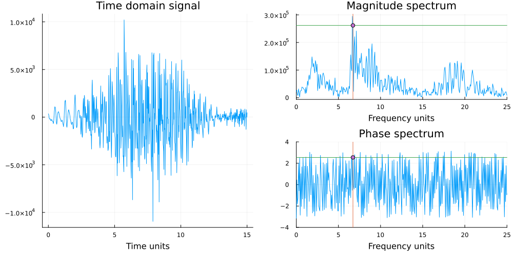
At this point, it might be instructive to take a minute and recall that we remarked in Lecture 01 that signals admit equivalent time and frequency domain representations and referred to this figure below. It is precisely via the Fourier transform that we get the frequency domain representation. Each coordinate on the right panel gives us three things: a frequency, a phase and a magnitude corresponding to a single sinusoid in the (possibly infinite) summation required to represent it.
We will skip the DTFT because of its limited practical application and in the next lecture we will arrive at equations equivalent to the ones shown in this lecture but without using imaginary numbers and complex mathematics.
In this lecture note, the intention was to provide a birds eye view of the theory of Fourier transforms and how it fits in the greater scheme of things. We have grossly neglected to discuss any implementations or calculations; both of which, hopefully will be addressed by homework, and in particular the latter which we will rectify with some worked out examples.
| [1] | No assumption is made that you have taken that class; if you are concurrently registered you will see the field axioms this semester. If not, ignore the statement. |
| [2] | Which BIOE205 isn't, so we must wrap up the discussion. |
| [3] | As you will see on this page, some of the "transforms", especially the first discrete ones, doesn't actually involve integrals, but it is common to refer to them all as transforms anyway. |
| [4] | For example, they are infinitely differentiable, admit Taylor series expansions, are orthogonal, etc. |