Lecture 03

Reading material: Section 1.4, 2.1 and 2.3 of the textbook.

Recap

Recall that last lecture we talked about:

sources of noise and variability in biological systems, some common examples of them and how to model and address them.
Gaussian models for noise and the essence of the central limit theorem.
types of systems including deterministic, stochastic, causal, non-causal, stationary, non-stationary, linear and nonlinear systems.
properties of some deterministic signals

In this lecture, we will continue the discussion to wrap up Chapter 1 material. Then we will move towards a discussion about processing of signals, including operations on signals, some common signals and their characterizations and constructions (both in theory & code).

Modeling biological systems
1. Analog(ue) approach
2. Systems approach
Elementary operations on signals
Constructing signals
1. Sinusoids
2. Manipulating sinusoids
Review of some basics regarding $\mathbb{C}$
1. Euler's formula

Modeling biological systems

The textbook discusses two different approaches to modeling biological systems as engineers. The first it calls the analog model and the second it calls the systems model. We briefly discuss the key themes in each here.

Analog(ue) approach

In this approach, we try to model the properties of the system using mechanical or electrical devices. For example, an early model of musculo-skeletal systems utilized nonlinear springs, contractile elements, and other such mechanical elements in series and parallel connections to mimic the properties and behavior shown in actual animal systems.

See Figure 1.23 in the textbook.

The key point here is: the differential equations which govern the behavior of the mechanical components used in the model, take the same (if simplified) form as those biological characteristic we seek to represent in the real system.

The model forces and velocities correspond to biological forces and velocities when mechanical elements are utilized to simulate biological mechanics. We could also do the same with electrical components if the same principle (that the defining dynamical equations are similar/identical) holds. As an example, we know from Ohm's law that a resistor provides a linear relationship between voltage & current. Then, using voltage as a stand-in for force (or pressure) and current for velocity, one can model features of the cardiovascular system with the resistance of the resistor mimicking the resistance provided by blood vessels to blood flow. Of course, blood vessels are not exactly the same as a plain old resistance since they are elastic and can expand. Thus one finds that the addition of a capacitance or the adoption of a nonlinear resistor is required to further capture such intricacies.

The "analog" in the title of this section thus is also rightly interpreted as an "analogous" approach and not just in the sense of analog vs. digital modeling.

Systems approach

In this approach, one does not seek to create models that mimic the exact behavior of a biological system with mechanical, electrical or pneumatic elements. Instead a more abstract approach is taken. Arguably, this is the more modern of the two approaches. In this conceptual framework, one wants to model the input-output behavior of different systems or system components. Rather than concentrate on the specifics of how each operation is implemented, the focus now is on accurately describing what the system does.

Since the key is now to describe accurately (often via differential equations) how the input or stimulus to the system is transformed into the output or response of the system, these models are frequently called transfer function models which are traditionally represented via system diagrams.

An important innovation in this approach is the separation of the process into a plant & a controller as well as the introduction of feedback to the system^[1]. Consider a simple system that must regulate or keep some variable $x$ of interest within an acceptable reference $r$ . Here $x$ could be the velocity of your car in cruise control mode or the temperature in your home when the thermostat is set to auto or your basic body temperature. In this setting, we can consider the ECU in the car or the thermostat in your home, or the autonomous nervous system to be the controller and the engine in the car or A/C unit in the home or our body itself to be the plant. It is the job of the controller to regulate the output of the plant.

In whichever system, one can consider the reference $r$ to be the input to the system controller: $60$ mph, $70 ^\circ$ F or $37 ^\circ$ C. In the systems model, this reference $r$ is compared to the current value or output coming from the plant and an error signal $e:=r-y$ generated using which the controller sends signals to the plant to modify its output. Since this output is then again measured, fed back into the system via the error signal we say that we have a feedback system (infact a negative feedback system, but that is for later lectures). The figure below illustrates this abstraction.

⚠️ Note

Here we transition to material of Chapter 2 of CSSB.

Elementary operations on signals

First we discuss about some elementary operations done on signals. All operations we discuss are visualized in the figure below.

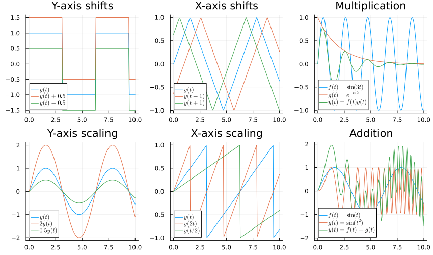
Y-axis shifts (vertical shift)

The first operation we are going to discuss is about $Y$ -axis shifts or vertical shifts.

Given a function $f(t)$ , its vertical shift is a new function $g(t) = f(t) + k$ . In other words, all the output values change by $k$ units. If $k$ is positive, the graph will shift up. If $k$ is negative, the graph will shift down.

In the figure $y(t) \pm 0.5$ is the vertically shifted versions of the original signal $y(t)$

X-axis shifts (horizontal/time shift)

The next operation is $X$ -axis shifting or time shifting of a signal. This means that the signal may be either delayed or advanced in the time axis.

Given a function $f(x)$ , a new function $g(x) = f(x-h)$ , where $h$ is a constant, is a horizontal shift of function $f(x)$ . If $h$ is positive, the graph will shift right. If $h$ is negative, the graph will shift left.

The figure above shows the time shifted version of the signal $y(t)$ , which is $y(t \pm h )$ , with $h=1$ .

\begin{aligned} y (t + 1) &\mapsto \textrm{negative shift (delayed signal)} \\ y (t - 1) &\mapsto \textrm{positive shift (advanced signal)} \end{aligned}

Multiplication

The next basic signal operation is Multiplication. In this case, amplitudes or output values of two signals are multiplied in order to obtain a new signal. Mathematically, this can be given as:

\begin{aligned} y(t) = f(t) \times g(t) \end{aligned}

In the figure, $y(t)$ is the product of two signals $f(t) = \sin(3t)$ and $g(t) = e^{-t/2}$ .

Y-axis scaling (amplitude scaling)

The process of rescaling the amplitude of a signal, i.e., the amplitude of the signal is either amplified or attenuated, is known as amplitude scaling. The amplitude scaling of a continuous time signal x(t) is defined as,

\begin{aligned} y(t) = A \cdot x(t) &\quad \textrm{where A is a constant} \\ \end{aligned}

In the above figure, as you can see, if $A > 1$ we have amplification of signal and if $A < 1$ we have attenuation of signal.

X-axis scaling (time scaling)

Time axis scaling of a signal $f(t)$ is also called reparametrization^[2] of $f(t)$ . Mathematically we write $g(t) = f(\lambda t)$ where $\lambda$ is a scalar constant. This in essence amounts to speeding up or slowing down of the signal. If $\lambda >1$ then the signal is sped up and if $\lambda<1$ then the signal is slowed down.

Addition

The addition of two signals is nothing but addition of their corresponding amplitudes. That is, if $f(t)$ and $g(t)$ are the two continuous time signals, then the addition of these two signals is expressed as $f(t) + g(t)$ .

The resultant signal can be represented as:

\begin{aligned} y(t) = f(t) + g(t) \end{aligned}

In the figure above, $f(t) = \sin(t)$ and $g(t) = \sin(t^2)$ .
The resultant signal is given by $y(t) = f(t) + g(t)$

Constructing signals

Next, we will be discussing how to construct signals. The first signal we will discuss is the sinusoid. In later lectures, we will discuss some other common signals.

Sinusoids

Sinusoidal signals are periodic functions which are based on the sine or cosine function. Note that the term sinusoid is a generic term for various curves or traces constructed using sines and cosines (which are of course related to each other)

The general form of a sinusoidal signal is

\begin{aligned} x(t) = A \sin(\omega t + \phi) \end{aligned}

Here $A$ , $\omega$ , and $\phi$ are parameters that characterize the sinusoidal signal. When $A=\omega=1$ and $\phi=0$ we get what we call a simple sinusoid.

Amplitude $A$ , of the signal determines how large the signal is in the dependent axis (height of the signal measured peak-to-valley). Specifically, the sinusoid oscillates between $+A$ and $-A$ absent any $y$ -axis shifts. Thus, $A$ acts like a $y$ -axis scaling factor on a simple sinusoid.
Frequency of the signal measures how fast the signal is in the time or independent axis. When it is measured in radians/second (recall that the sine function takes an angle as input) it is represented by $\omega$ (known as angular frequency). The frequency $f$ , in Hertz (Hz) provides the number of complete cycles that the sinusoid repeats in one second. The duration of each cycle is called the period ( $T$ ) of the sinusoid.

Mathematically, the frequency (in Hertz) of a sinusoid is simply the inverse of its period and also related to the angular frequency as follows:

f = \frac{1}{T} \qquad f = \frac{\omega}{2\pi} \qquad \omega = 2 \pi f

Phase ( $\phi$ ) of sinusoid causes a sinusoid to be time or $x$ -axis shifted.

Since frequency is the inverse of the period and for a simple sinusoid

\omega=1

, we have that

\omega = 2\pi f \implies f = \dfrac{1}{2\pi} \implies T = 2 \pi

The unit is in seconds. That is, the simple sinusoid completes one full cycle in

2 \pi

seconds.

Constructing and plotting sinusoids

Mathematically, constructing a sinusoid of a given amplitude and frequency is easy. We just plug in the right numbers.

Let's parse this.

Clearly $A=3$ to have an amplitude of 3 units. Thus our starting guess for the form of the signal is $y(t) = 3\sin(\omega t)$ . Now 12 cycles every minute implies $f = 12/60$ Hz. Thus our signal becomes $y = 3 \sin ( 2\pi/5 t)$ , i.e. $\omega = 2\pi/5$ . Since we need the signal to start at 1.5V, we can try a y-axis shift: $y(t) = 3\sin(\omega t) + 1.5$ . However this signal violates the given constraint (why?).

Thus we should try a different strategy. Let's introduce a phase shift: $y(t) = 3 \sin(\omega t + \phi)$ . Then solve for $y(0) = 1.5 = 3\sin(\phi)$ to get that the required signal is:

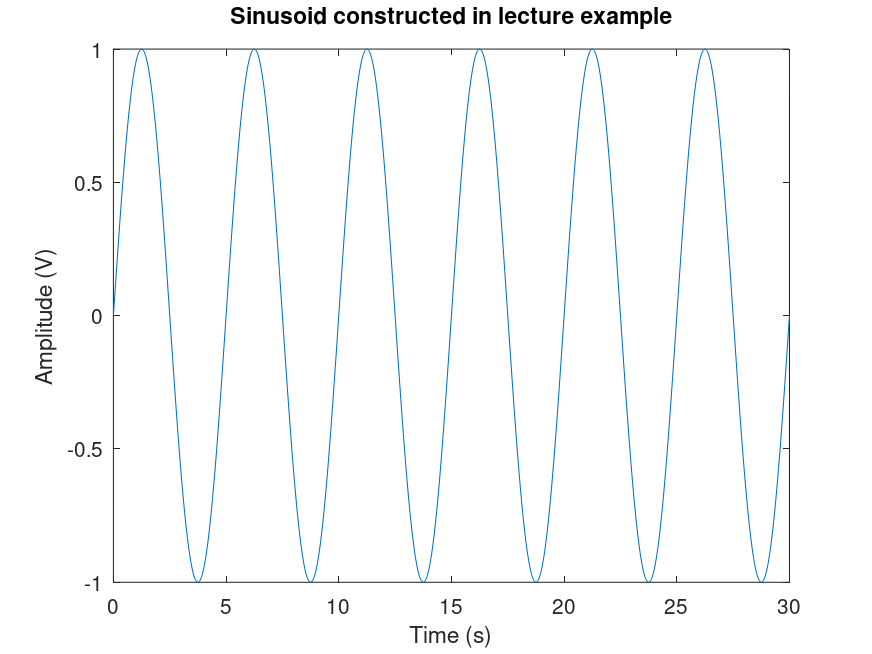
y(t) = 3\sin(\omega t + \phi) \qquad \omega = \dfrac{2\pi}{5} \qquad \phi = \dfrac{\pi}{6}

While mathematically constructing a sinusoid is straightforward as we have seen above, visualizing one using a computer involves a bit more work. First, recall that digital signals are not continuous time signals; but rather, they are discretized using some sampling scheme. Therefore, the first task we must complete is to define what the sampling frequency will be for our signal. Suppose we want to plot 30 seconds of the above example signal (how many cycles would you expect to see?) and we make 50 measurements every second. Thus we have,

fsample = 50;
t0 = 0; 
tf = 30;
fsignal = 2*pi/5;

where fsample is the sampling frequency and fsignal is the frequency of the desired signal and t0, tf denote the interval over which we wish to visualize the signal. Next we generate the time vector t=t0:1/fsample:tf and the plot it. The whole code is shown below

fsample = 50;
t0 = 0; 
tf = 30;
fsignal = 2*pi/5;

t = t0:1/fsample:tf;
y = sin(fsignal*t);
plot(t, y)
xlabel("Time (s)")
ylabel("Amplitude (V)")
title("Sinusoid constructed in lecture example")

Note that we add some styling elements using xlabel and ylabel commands.

Manipulating sinusoids

It is often convenient to analytically manipulate sine/cosine waves. To add two sine waves of the same frequency just add their amplitudes together.

y_k = a_k \sin (\omega t) \implies \sum \limits _k y_k = \left( \sum \limits _k a_k \right) \sin (\omega t)

The same applies to cosines.

y_k = a_k \cos (\omega t) \implies \sum \limits _k y_k = \left( \sum \limits _k a_k \right) \cos (\omega t)

Therefore, to add a sine wave to a cosine wave, we must first write them both using the same function; either sine or cosine. For example, we already noted that

\cos(t - \pi/2) = \sin(t)

and so

\cos(t) + \sin(t) = \cos(t) + \cos(t - \pi/2)

. But this means we will need to address how to deal with phase differences:

c_1 \cos(\omega t) + c_2 \cos (\omega t - \phi) = \qquad ??

Now it becomes convenient to represent a general sinusoid

y(t) = A \cos(\omega t + \phi)

in terms of pure sines & cosines. This can be done using

\cos(x - y) = \cos(x) \cos(y) + \sin(x) \sin(y)

Answer: Note that the (1) directly gives

\begin{aligned} A \cos (\omega t + \phi) &= A\cos(\omega t) \cos(-\phi) + A\sin(\omega t) \sin(-\phi) \\ &= A\cos(\phi)\cos(\omega t) - A\sin(\phi) \sin(\omega t) \end{aligned}

A similar relation exists for converting a sinusoid in terms of the sine function into a sum of pure sines and cosines as well. Therefore, now we have the procedure to analytically add sinusoids.

To add two sinusoids,

S_k\sin(\omega t + \phi_k)

C_k \sin(\omega t + \phi_k)

convert them to expressions involving pure sinusoids, then add sines to sines and cosines to cosines, converting back to a single sinusoid if desired.

Review of some basics regarding $\mathbb{C}$

We will have the opportunity to work with Euler's formula and the complex numbers as well as complex exponentials in this course. Therefore at this stage it is instructive to review the basic laws of logarithms and exponents. This should be very familiar material.

For a real number $a \neq 0$ we define, $a^0:=1$ . Then, for two real numbers $a, b$ and two integers $m, n$ the following laws hold.

$a^m a^n = a^{m+n}$
$(a^m)^n = a^{mn}$
$(ab)^{mn} = a^mb^n$
$a^{-k} = \dfrac{1}{a^k}; \qquad a \neq 0$
$a^{1/n} = \sqrt[n]{a}$

The logarithm is defined as an operation using the following:

Definition: (Logarithm) We say

y = \log _a x

if and only if

x = a^y

for positive nonzero

a

One should read the operation $\log _a x$ as "logarithm to the base $a$ of $x$ ". When the base, $a=e$ , we replace the notation $\log$ with $\ln$ (natural logarithm)^[3].

From the above definition it is true that:

x = a^{\log _a x} \qquad \textrm{and} \qquad y = \log _a (a^y)

Then the following properties hold as a result:

$\log _a (xy) = \log x + \log y$
$\log _a (x^y) = y \log _a x$
$\log _a (x/y) = \log_a x - \log_a y$

We have from the first observation in (1) that we can write for some valid base

a

x = a^{\log _a x} \qquad \textrm{and} \qquad y = a^{\log _a y }

Then,

\begin{aligned} x y = a^{\log _a x} a^{\log _a y} &= a^{\log _a x + \log _a y} \\ xy = a^{\log _a (xy)} &= a^{\log _a x + \log_a y} \end{aligned}

The first line uses the properties of exponents. In the second line, the first equality arises by doing

z = a^{\log _a z}

with

z=xy

Since the second equality in the last line above has the same base then the two exponents must be equal. Thus follows the identity.

The other identities are left as an exercise.

We assume the class is familiar with complex numbers and operations on them. Recall that while real numbers $\mathbb{R}$ are one dimensional, the complexes $\mathbb{C}$ are two dimensional, having both a real coordinate and an imaginary coordinate. All complex numbers therefore can be written in a Cartesian form $z = (a, b)$ (often written $z = a+ib$ ) and as well as a polar form $z = (r, \theta)$ .

Appendix F in CSSB has a primer on complex arithmetic which you should peruse if you haven't seen them in a long time.

Answer: Left as an exercise. Might help to draw out a diagram and recall some basic trigonometry.

Euler's formula

Euler's formula indicates an essential and deeply profound relationship between the Polar and Cartesian forms via Euler's constant $e$ causing 19th century Harvard mathematician Benjamin Peirce to remark (after proving a particular version of it):

Gentlemen, that is surely true, it is absolutely paradoxical; we cannot understand it, and we don't know what it means. But we have proved it, and therefore we know it is the truth.

Let us therefore prove it, starting with only the supposition that a complex number as an exponent to $e$ should return a complex number^[4] and examining what calculus can tell us.

Let $e^{ix}$ , being a complex number, have some polar representation:

e^{ix} = r \left( \cos \theta + i \sin \theta \right)

Differentiate both sides (with respect to $x$ and not assuming anything about $r$ or $\theta$ ) and follow the product rule of calculus:

i e^{ix} = \left( \cos \theta + i \sin \theta \right) \dfrac{dr}{dx} + r \left( - \sin \theta + i \cos \theta \right) \dfrac{d\theta}{dx}

Put definition (3) back into the left hand side of (4). Then we have,

\begin{aligned} ir \left(\cos \theta + i \sin \theta \right) &= \left( \cos \theta + i \sin \theta \right) \dfrac{dr}{dx} + r \left( - \sin \theta + i \cos \theta \right) \dfrac{d\theta}{dx} \end{aligned}

Expanding out and collecting the real and imaginary parts we get:

\begin{aligned} r \cos \theta &= \sin \theta \dfrac{dr}{dx} + r \cos \theta \dfrac{d\theta}{dx} \\ -r \sin \theta &= \cos \theta \dfrac{dr}{dx} - r \sin \theta \dfrac{d\theta}{dx} \end{aligned}

For equality to hold we must have:

\dfrac{dr}{dx} = 0 \qquad \textrm{and} \qquad \dfrac{d\theta}{dx} = 1

Therefore $r$ is a constant and $\theta = x + C$ where $C$ is another constant and we have:

e^{ix} = r \left( \cos (x+C) + i \sin (x+C) \right)

Considering

e^{i0}=1

for

x=0

in the above, we get

1 = r \left( \cos C + i \sin C \right)

Once again collecting the real and imaginary parts we get that the above system of two equations has two solutions. Since the magnitude

r

is restricted to be non-negative we choose the solution with

r=1

and

C=2n\pi

for

n \in \mathbb{Z}

.
Thus for

n=0

we get Euler's formula:

e^{ix} = \cos x + i \sin x

Note: It is indeed $2 \pi$ periodic.

Now let us use it a couple of times.

Answer:
(a) We can simply use

e^{ix} = \cos x + i \sin x

with

x=1

. Thus,

e^i = \cos 1 + i \sin 1

(b) Recall that

3 = e^{\ln 3}

and therefore

3^i = \left( e^{\ln 3} \right)^i

. Therefore,

3^i = e^{i\ln(3)} = \cos (\ln 3) + i \sin (\ln 3 )

[back]

[1]	The term plant is a relic from the old times when these concepts were first introduced in the setting of large industrial production plants (often for chemicals).

[2]	Technically this encompasses arbitrary changes to the timeline $t' = \phi(t)$ but we don't discuss that here.

[3]	It is natural in many senses that are beyond the scope of the course; but it suffices to note that $e$ is a very important mathematical constant on par with $\pi$ .

[4]	A much more natural assumption than Appendix A in CSSB which admittedly seems to start out of nowhere.

CC BY-SA 4.0 Ivan Abraham. Last modified: February 05, 2023. Website built with Franklin.jl and the Julia programming language. Curious? See familiar examples.