Julia
Are you curious about the Julia language that was used to create the course webapage? Julia is an up and coming language that is being widely adopted: both in academia, industry and elsewhere around the world. It will not replace MATLAB (or Python) any time soon, but it is being actively developed with a lot of interesting & promising features.
This page shows a few examples from the text converted to Julia code. Compare the outputs with the textbook images and the code samples to get a feel for Julia if interested.
To see more of Julia in action check out this course from MIT.
Example 1.2 - MATLAB Code
clear all, close all;
N = 100;        	% Number of pixels per line and number of lines
x = (1:N)/N;      	% Spatial vector
y = sin(8*pi*x);	% Four cycle sine wave
for k = 1:N
    I(k,:) = y;		% Duplicate 100 times
end
pcolor(I);              % Display image
colormap(bone);      	% Use a grayscale color map
Example 1.2 - Julia Code
# This is Julia code; it will not run in MATLAB or Python.
using Plots

N = 100;
x = (1:N)/N;
y = sin.(8π.*x);
I = [y for _ in range(1,100)];
heatmap(hcat(I...)', c=:bone)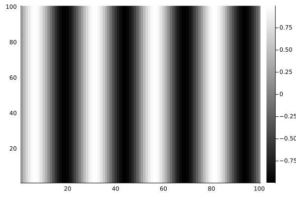
Example 1.3 - MATLAB Code
% Example 1.3  Example to apply some mathematical and threshold operations
%   to an MR image %  of the brain.

clear all; close all;
load brain;         		% Load image
subplot(2,2,1);             	% Display the images 2 by 2
pcolor(I);           		% Display original image
colormap(bone);             	% Grayscale color map
caxis([0 1]);        		% Fix pcolor scale
title('Orignal Image');

subplot(2,2,2);
I1 = I + .3;			% Brighten the image by adding 0.3
pcolor(I1);           		% Display original image
colormap(bone);             	% Grayscale color map
caxis([0 1]);        		% Fix pcolor scale
title('Lightened');

subplot(2,2,3);
I1 = 1.75*I;			% Increase image contrast by multiplying by 1.75
pcolor(I1);           		% Display original image
colormap(bone);             	% Grayscale color map
caxis([0 1]);        		% Fix pcolor scale
title('Contrast Enhansed');

subplot(2,2,4);
[r, c] = size(I);           	% Get image dimensions
thresh = 0.25;			% Set threshold
for k = 1:r
    for j = 1:c
        if I(k,j) < thresh 	% Test each pixel separately
            I1(k,j) = 1;	% If low make corresponding pixel white (1)
        else
            I1(k,j) = 0;	% Otherwise make it black (0)
        end
    end
end
pcolor(I1);           		% Display original image
colormap(bone);             	% Grayscale color map
caxis([0 1]);        		% Fix pcolor scale
title('Thresholded');
Example 1.3 - Julia Code
# This is Julia code; it will not run in MATLAB or Python.
using Plots, MAT

path = "_assets/matlab/"
I = read(matopen(joinpath(path,"brain.mat")), "I")
p11 = heatmap(I, c=:bone, title="Original Image", clims=(0,1))
p12 = heatmap(I .+ 0.30, c=:bone, title="Lightened", clims=(0,1))
p21 = heatmap(I .* 1.75, c=:bone, title="Contrast Enhanced", clims=(0,1))

I1 = zero(I)
I1[I .< 0.25] .= 1
p22 = heatmap(I1, c=:bone, title="Thresholded", clims=(0,1))

l = @layout [a b; c d]
plot(p11, p12, p21, p22, layout=l, size=(800,600))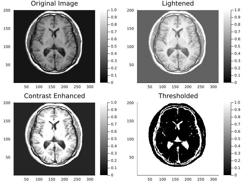
Example 2.15 - MATLAB Code
function [rxy lags] = crosscorr(x,y)
	lx = length(x);		% Assume both the same length
	maxlags = 2*lx - 1;     % Compute maxlags from data length
	x = [zeros(1,lx-1) x zeros(1,lx-1)]; % Zero pad signal x
	for k = 1:maxlags
    		x1 = x(k:k+lx-1);         % Shift signal
    		rxy(k) = mean(x1.*y);     % Correlation (Eq. 2.30)
    		lags(k) = k - lx;         % Compute lags
	end
end
% Example 2.15 Find the correlation between the EEG signal
% and sinusoids ranging from 1 to 40 Hz in 1.0 Hz increments.
clear all; close all;
load eeg_data1; % hide
N = length(eeg); % Number of points
fs = 50; % Sampling frequency of data
f = (1:.5:25); % Frequency of reference signals
t = (0:N-1)/fs; % Time vector from 0 (approx.) to 2 sec.
for k = 1:length(f)
x = cos(2*pi*f(k)*t); % Generate reference signal
rxy = crosscorr(x,eeg); % Compute crosscorreltion
max_corr(k)= max(rxy); % Find maximum correlation
rxy_M = xcorr(x,eeg,'biased'); % Find crosscorrelation MATLAB
max_corr_M(k) = max(rxy_M); % MATLAB's max correlation
end
plot(f,max_corr,'k'); hold on;
plot(f,max_corr_M,'*k');
xlabel('Reference Signal Frequency (Hz)','FontSize',14);
ylabel('Max Correlation','FontSize',14);Example 2.15 - Julia Code
# This is Julia code; it will not run in MATLAB or Python.
using Plots, StatsBase, MAT

function crosscorr(x, y)
    lx, rxx, lags = length(x), AbstractFloat[], Integer[]
    x = vcat(zeros(lx-1), x, zeros(lx-1))
    lags_ranges = [(k-lx, k:k+lx-1) for k=1:2*lx-1]

    foreach(lags_ranges) do (lag, range)
	    push!(rxx, mean(x[range].*y))
	    push!(lags, lag)
    end
    return rxx, lags
end

N, fs = length(eeg), 50  # Length, sampling frequency of data
t = (0:N-1)/fs           # Time vector from 0 (approx.) to 2 sec.
freqs=1:0.5:25
refs = [cos.(2π.*f.*t) for f=freqs]       # Reference signals
result = zip(refs, map(x -> crosscorr(eeg, x), refs))

max_corr, max_corr_M = [], []
foreach(result) do (ref, (rxx, lags))
	push!(max_corr, maximum(rxx))
	push!(max_corr_M, maximum(crosscov(eeg, ref, lags, demean=false)))
end

xlabel = "Reference Signal Frequency (Hz)"
ylabel = "Max correlation"
plot(freqs, max_corr, label="Manual", xlabel=xlabel, ylabel=ylabel)
plot!(freqs, max_corr_M, markershape=:circle, ls=:dot, label="StatsBase")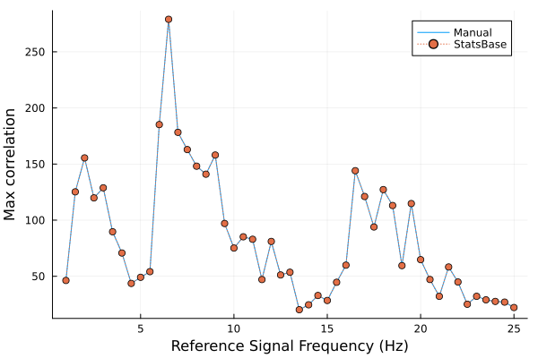
Example - Sierpinski Triangle
using Plots, Base.Iterators, Statistics

function sierpinski_triangle(coords,lvl,fig)
	lvl==0 && return fig
	plot_coords(c) = map(first, c), map(last, c)
	new_cs(c) = map(mean, plot_coords(c))
	ln, mn, rn = [new_cs(x) for x in take(partition(cycle(coords),2),3)]

	foreach(product(coords, coords)) do (i, j)
		plot!(fig, plot_coords([i,j]), axis=false, legend=false)
	end

	sierpinski_triangle([coords[1], ln, mn],lvl-1,fig)
	sierpinski_triangle([ln, coords[2], rn],lvl-1,fig)
	sierpinski_triangle([mn, rn, coords[3]],lvl-1,fig)
end

init = [(0,0),(0.5,1),(1,0)]
sierpinski_triangle(init, 6, plot(size=(800,600)))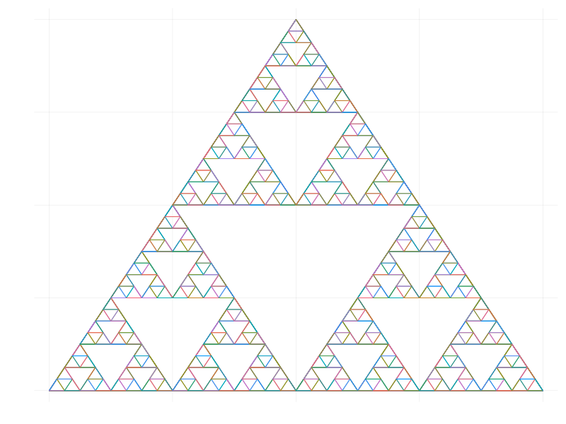
CC BY-SA 4.0 Ivan Abraham. Last modified: May 21, 2023.
Website built with Franklin.jl and
the Julia programming language.
Curious? See familiar examples.