Lecture 02

Reading material: Section 1.3 - 1.4 of the textbook.

Recap

Last time we talked about a few systems concepts including

what constitutes a system
how systems communicate within themselves and with the outside world using signals
how we can categorize signals
how we can represent signals in the frequency domain or the time domain and finally
how images can be interpreted as two dimensional signals.

Today we will cover some more introductory material related to systems and signals including noise in measurements, types & sources of noise, the central limit theorem and why it is useful etc.

Noise & variability in systems
1. Common forms of electrical noise
Gaussian additivity & central limit theorem
1. Estimating PDF from given data
Types of systems
Other classifications

Noise & variability in systems

This course primarily deals with signals and systems and in this context the word noise signifies components in a signal that are either detrimental to our signal processing objective or simply unwanted. Recall that signals encode information by variations in their energy content. However, not all variation contains useful information, and it is precisely this unwanted variation that we term noise.

Noise can arise in a biological system primarily from four sources.

Physiological variability/indeterminacy: This is noise that enters a system simply because of the fact that biological processes do not happen in isolation and can influence each other. Therefore, the information we want can be based on measurements subject to influence from processes, that are not material to our objective. Noise due to physiological indeterminacy is one of the hardest forms of noise to account for in the analysis.
Environmental noise: These are sources of noise that may be internal or external to the system. As an example of the former, a fetal ECG signal can be corrupted or confused by unavoidable input from the mother's cardiovascular system. For an example of an external noise, consider x-ray films which can be sensitive to background or other sources of radiation. Environmental noise sources can be controlled to some extent by careful experiment design.
Measurement noise: Whenever there is a measurement made, there is also an opportunity for noise to enter the system. This is typically due to the properties or characteristics of the transducer. In particular, this noise is generated by the transducer responding to unintended or undesired energy modalities. For example, ECG measurements made by attaching electrodes to the skin respond not only to cardiac electrical activity but also to mechanical movement (a.k.a motion artifact ).
Electrical noise: This source of noise is perhaps amongst the most well understood ones. Electrical noise refers to noise added to the signal by the characteristics of the electrical circuitry that transmits or carries the signal including semiconductors, inductors and other circuit elements.

Table 1.4 from the textbook summarizes this information.

Source	Cause	Potential Remedy
Physiological indeterminacy	Measurement indirectly related to variable of interest	Modify overall approach
Environmental (internal or external)	Other sources of similar energy	Apply noise cancellation; Alter transducer design
Measurement artifact	Transducer responds to other energy sources	Alter transducer design
Electronic	Thermal or shot noise	Alter transducer or electronic design

Common forms of electrical noise

The forms of electrical noise we can characterize are:

Thermal noise: related to the resistive elements in the circuit and depends on resistance, temperature and bandwidth

V_j = \sqrt{4kT \cdot R \cdot BW}

where $k$ is the Boltzmann constant, $T$ is the temperature in Kelvin, $R$ is the resistance in Ohms and $BW$ is the bandwidth in Hertz.

Shot noise: related to the semiconducting elements in the circuit and depends on baseline current and bandwidth

I_s = \sqrt{2q \cdot I_d \cdot BW}

I_j = \sqrt{4kT \cdot \dfrac{BW}{R}}

When multiple noise sources are present, their voltage or current contributions add as the square root of the sum of the squares. For voltages,

V_T = \sqrt{V_1^2 + V_2^2 + V_3^2 \dots }

At the provided temperature the term

4kT = 1.712 \times 10^{-20} J

. The elementary charge of an electron is

1.602 \times 10^{-19}

Coulomb^[1]. Let the current in the circuit be

I

. Then the total current noise

i_T

is given as

\begin{aligned} i_T &= \sqrt{i_R^2 + i_D^2} \\ &=\sqrt{ \left(\sqrt{4kT \cdot \dfrac{BW}{R}} \right)^2 + \left( \sqrt{2q \cdot I \cdot BW} \right) ^2 } \\ &=\sqrt{\left(\dfrac{4kT}{R} + 2q I \right) BW } \end{aligned}

The calculation works out to be

\approx 8 \times 10^{-8}

amps.

Gaussian additivity & central limit theorem

Since noise in a signal is random variations that are not of interest to us, it is helpful to have methods to characterize it. Unfortunately, the exact statistical properties of the individual sources of noise are usually extremely hard to fathom. Nevertheless, the Central Limit Theorem ^[2] (roughly) states that the properly normalized sum of many independent random variables tends toward the Gaussian distribution regardless of the distribution of the individual random variables. This is very useful to us because it means in the long run the methods that apply to Gaussian distributions can also apply to the noise terms. One key property of interest here is the additivity of Gaussian random variables. In other words, for most of our purposes, we can model noise in our signal as a Gaussian random variable entering the system additively.

Recall, the probability distribution function of the Gaussian distribution is given by:

p(x) = \dfrac{1}{\sigma\sqrt{2\pi}} \exp\left( \dfrac{-(x-\mu)^2}{2\sigma^2} \right)

Estimating PDF from given data

One frequent exercise we perform when we get data is to try and estimate what the probability distribution function (PDF) of the data looks like. A typical way to do this is to plot its histogram. The following code shows how to plot histograms in Python (see Example 1.4 in the textbook for the MATLAB version).

N = 20000                   # Number of data points
nu_bins = 40                # Number of bins

y = np.random.randn(1,N)                # Generate random Gaussian noise
ht, xout = np.histogram(y,nu_bins)      # Calculate histogram
ht = ht/max(ht)                         # Normalize histogram to 1.0

# Setup figure & subplots
fig, (top, bot) = plt.subplots(2,1, figsize=(8,6), constrained_layout=True)

# Plot as bar graph (use color)
top.bar(xout[:-1], ht, width=0.1, edgecolor='black', align='edge')
top.set_xlabel('x')
top.set_ylabel('P(x)')
top.set_ylim(0, 1.2)
top.set_title('Gaussian noise (randn)')

y = np.random.rand(1,N)                 # Generate uniform random samples
ht, xout = np.histogram(y,nu_bins)      # Calculate histogram
ht = ht/max(ht)                         # Normalize histogram to 1.0

# Plot as bar graph (use color)
# bot.hist(xout[:-1], xout, weights=ht, width=0.01, edgecolor='black')
bot.bar(xout[:-1], ht, width=0.01, edgecolor='black', align='edge')
bot.set_xlabel('x')
bot.set_ylabel('P(x)')
bot.set_ylim(0, 1.2)
bot.set_title('Uniform noise (rand)')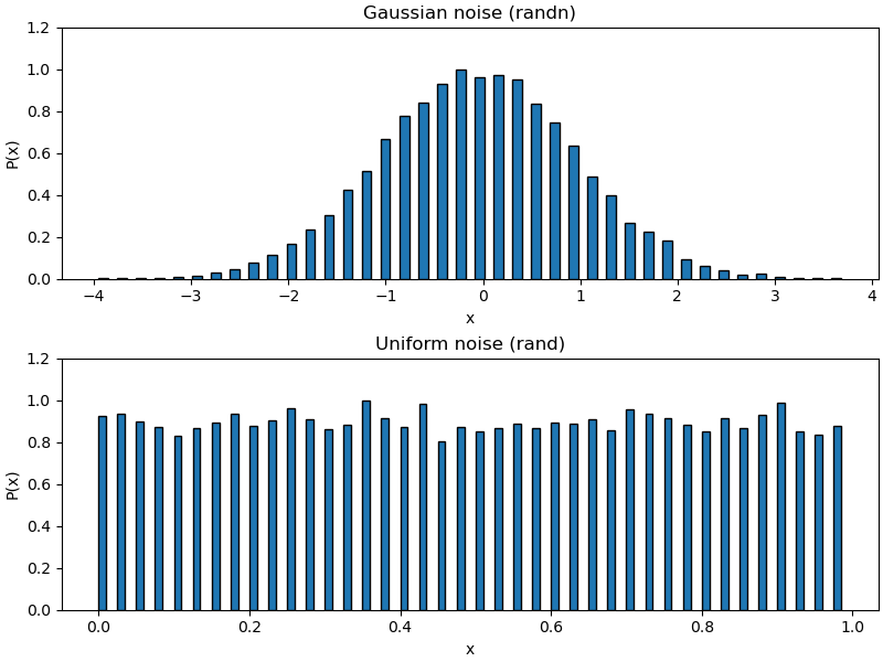

The top plot shows a histogram of N=20000 points generated by the np.random.randn function (equivalent of MATLAB's randn) while the bottom shows the same for the np.random.rand function (equivalent of MATLAB's rand).

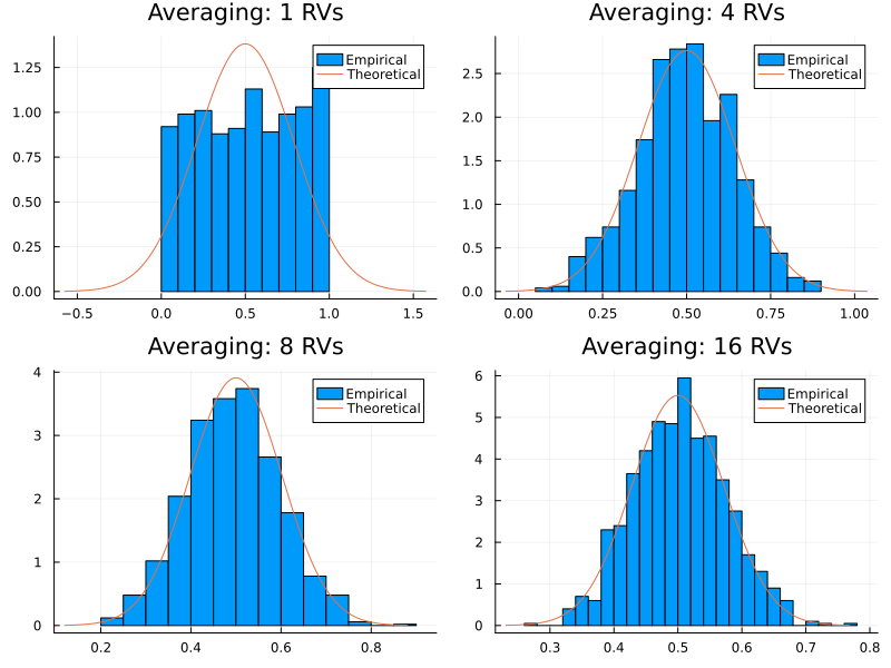
Example: The below plot shows the central limit theorem in action. The top left plot shows the probability distribution function (PDF) of 20000 random variables (RVs) drawn from an uniform distribution on the interval $[0, 1]$ . The subsequent plots show the PDF as 2, 8 and 16 RVs are averaged together. Clearly the PDF is tending towards the normal distribution.

Update (advanced)

If you are interested in knowing more about the Central Limit Theorem I highly recommend watching this excellent video by Grant Sanderson which was released after we covered this lecture:

Types of systems

Depending on the behavior of the signals generated by a system, engineers often classified the systems into various kinds. We go over a few of these now.

Deterministic versus stochastic systems

A signal is said to be deterministic if there is no uncertainty with respect to its value at any instant of time. In other words, a signal is deterministic if it can be represented by a system of ordinary differential equations^[3]. For example, sine waves, cosine waves, square waves, etc. are all deterministic as their value at any instant of time can be predicted with perfect accuracy by only knowing their frequency, amplitude and phase. These kind of signals show no randomness in their behaviour and hence makes it possible to predict their future behavior from the past values.

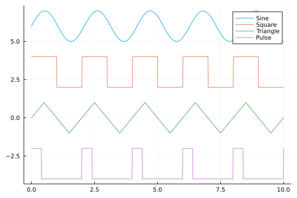
A simpler subtype of deterministic signals are the periodic signals. Periodic signals are repetitive in nature and often are simply characterized by the shape of their waveform and the period with which the waveform repeats. The figure below shows a few kinds of periodic signals.

In contrast to deterministic signals, stochastic signals are signals that have some element of randomness to them and therefore frequently serve as models of noise. These signals involve a certain degree of uncertainty in their values and thus cannot be described by standard ordinary differential equations. Rather, they are better characterized from a probabilistic framework and invoke the theory of random processes and variables.

Chaotic signals and systems

One subclass of deterministic systems that are frequently misunderstood are the so called chaotic systems. Chaotic systems, unlike what the name seems to imply, are not stochastic or random at all. They are, in fact, completely determined by their differential equations. However they are extremely sensitive to initial conditions and/or changes in their parameters; so much so that change in a parameter by 1 part in 10,000 drastically changes system behavior.

One of the most famous examples of a chaotic system is the so called logistic map, a simple population model which shows wildly different behavior depending on the value a certain parameter takes. The equation for the logistic map is deceptively simple:

x_{n+1} = rx_n(1 - x_n)

where $x$ is a variable representing the population as a fraction of the maximum possible (always taken to be 1) and $r$ is a growth rate. Therefore one can interpret $rx_n$ as growth dependent on the current population, while the $(1-x_n)$ term is present to account for capacity constraints, i.e. population cannot grow unbounded forever.

The plot below shows the difference in system behavior for different values of $r$ .

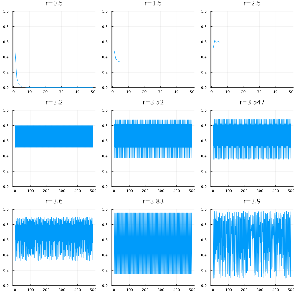
As you can see:

For $0 < r < 1$ , the population eventually dies out (see top-left plot).
For values in the range $1 < r < 2$ , the population reaches a steady state value of $\frac{r-1}{r}$ independent of the value of $x(0)$ (top-middle plot).
For $0 < r < 3$ , the same steady state is reached but now with some transient behavior in the beginning (top-right plot).
For $3 < r < r + \sqrt{6}$ , the steady state oscillates between two values (middle-left plot)
For $3 + \sqrt{6} < r < \approx 3.54409$ , the steady state oscillates between four different values (center plot) ... and so
... there follows a regime of period doubling up until $r \approx 3.56995$ which is the onset of chaos (bottom left plot) where the behavior is no longer as well ordered or predictable while the describing equation (2) remains still completely deterministic ^[4].

For more information on the logistic map, see here, which is a tool that allows you to experiment with various parameters in the logistic map system.

Chaos theory is a deep and rich topic within the field of dynamical systems and could serve as a topic for a semester long course in itself

\dots

and so we will end our discussion on it with this lecture.

Deterministic signals: periodic, aperiodic, and transient behaviors

Brushing aside chaotic systems for now, let us return to some properties and definitions that serve to characterize simpler deterministic systems.

Periodic signal
We briefly mentioned periodic signals above. More precisely, a periodic signal is one that repeats the sequence of values exactly after a fixed length of time, known as the "period". The mathematical property that is obeyed by a periodic signal is:

x(t) = x(t+T)

A period $T$ , is defined as the amount of time required to complete one full cycle. The reciprocal of the time period of the periodic signal is called the frequency $f$ of the signal, i.e.

f = \dfrac{1}{T}

Frequency can be expressed in either radians or Hertz and are related by $2\pi$ :

\omega = 2 \pi f

Sine waves are classic examples of periodic signals.

Aperiodic signals
Aperiodic signals (using the textbook definition) are signals that have bounded support. That is to say, they exist for a definite period of time and are treated as being zero outside that interval of existence. Therefore operations on aperiodic signals need only be applied to their finite, non-zero segments. One mathematically convenient way to view aperiodic signals is as periodic signals where the period goes to infinity.

Transient signals
Transient signals are ones that do not repeat in time, but also do not have a bounded support. Examples given in the textbook include step functions, signals that reach a steady state asymptotically as well as signals that grow ever larger on their domain.

❗ Caution

Note: The terminology used in the textbook to describe all signals with unbounded support as transient is not standard. In electrical engineering, mathematics & physics, more often we call transient signals as ones that die out with time. So within this context, the third bullet above (in describing the logistic map outputs) refers to a plot with a transient portion in the very beginning.

Other classifications

Linear vs. nonlinear systems

Linearity is a concept that encapsulates the notion of "proportionality in response", i.e., the output should be proportional to the input. Mathematically this is expressed as follows: A function/signal/operator, $f$ , is said to be linear if for any $x, y$ in its domain:

f(x + \lambda y) = f(x) + \lambda f(y)

It is easy to see then that the usual sine and cosine functions are not linear in nature since $\sin(2x) \neq 2\sin(x)$ and the same is true for the cosine.

Or are we?
We cheated a bit and split/distributed the

\dfrac{d}{dt}

operation over addition. How do we know we allowed to do this? The answer is to use the limit definition of differentiation.

h'(x) := \lim \limits _{\epsilon \to 0} \dfrac{h(x+\epsilon) - h(x)}{\epsilon}

Let our $h(x) = f(x) + k g(x)$ . So we have,

\begin{aligned} h'(x) &= \lim \limits _{\epsilon \to 0} \dfrac{f(x+\epsilon) +k g (x + \epsilon) - f(x) - kg(x)}{\epsilon} \\ & = \lim \limits _{\epsilon \to 0} \dfrac{f(x+\epsilon) - f(x) +k g (x + \epsilon) - kg(x)}{\epsilon} \end{aligned}

where we have just rearranged the terms. Next we split the fraction and move the limit inside (we assume we know we can distribute it over addition):

\begin{aligned} h'(x) &= \lim \limits _{\epsilon \to 0} \dfrac{f(x+\epsilon) - f(x)}{\epsilon} + \dfrac{k g (x + \epsilon) - kg(x)}{\epsilon} \\ & = \lim \limits _{\epsilon \to 0} \dfrac{f(x+\epsilon) - f(x)}{\epsilon} + k \cdot \dfrac{g (x + \epsilon) - g(x)}{\epsilon} \\ & = \lim \limits _{\epsilon \to 0} \dfrac{f(x+\epsilon) - f(x)}{\epsilon} + k \cdot \lim \limits _{\epsilon \to 0} \dfrac{ g (x + \epsilon) - g(x)}{\epsilon} \end{aligned}

But the above is just the definition of differentiation. Thus,

\begin{aligned} h'(x) =\dfrac{d}{dx}f(x) + k \dfrac{d}{dx} g(x) = f'(x) + kg'(x) \end{aligned}

and differentiation is indeed a linear operator. Integration is also linear but showing that requires a bit more mathematical machinery than we have at our disposal in this course. It is left as an exercise for the mathematically inclined.

The next bit describes one way to examine if a system is linear or not.

In truth, most real systems will likely exhibit nonlinearity if they are tested over a wide enough range of inputs. Example 1.7 of the textbook takes a few sinusoids of different amplitudes as input to an unknown system and then examines the output relative to the input as a test for linearity. Make sure you understand the example well.

⚠️ Note

It is common to call equations like

y = 5x + 3

as the equation of a line and thus "linear". We invite the reader to think if the function

y(x) = 5x +3

is actually linear or something else.

Time-invariant vs. non-stationary

Time-invariant systems are one where the equations describing the system dynamics do not change with time. We already saw one example of such a system (albeit in discrete time) with the logistic map above. Here, for any fixed value of $r$ , the population described by the system varies with time; however its basic statistical properties do not; precisely because the mathematical equation describing the system does not change with time. While the logistic map is a nonlinear equation, in general parlance, time invariant systems refer specifically to linear time invariant systems & signals. As such, these signals exhibit the following mathematical property: if $f$ is a linear function of $x(t)$ then for any $T$ , the signal $y(t) = f(x)$ is time invariant if $y(t-T) = f(x(t-T))$ .

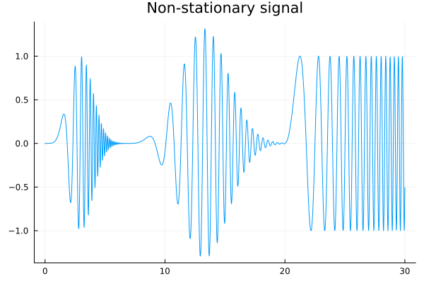
On the other hand, signals exist whose statistical properties change with time. These statistical properties may include mean, variance, correlations etc. Such signals are called nonstationary signals; if these signals have defining equations, those change over time. More often than not, it is extremely hard to find equations that can adequately describe the dynamics of an observed nonstationary signal. Nonstationarities present a moving target to any analysis approach - if dealt with at all, it is usually on an ad hoc basis, depending strongly on the type of nonstationarity and are the subject of later chapters/lectures. The figure below is an example of a nonstationary signal. The signal properties are markedly different depending on the time interval it is observed across.

Answer: Left as an exercise.

Causal and non-causal systems

Causality is a general principle that implies that the future cannot influence its past; or in other words, in terms of systems and biological systems, the stimulus must precede the response. All physical systems are necessarily causal in nature. Mathematically, we represent explicitly the causal nature of a signal by setting $y(t) = 0$ for $t < t_{0}$ . Thus, every system starts at some initial state $y(t_0)$ associated with its initial time $t_0$ . Often by convention we take $t_0=0$ . Furthermore, any indices/arguments or time values appearing on the right side of a system equation must be lower in value than the ones appearing on the left side in a causal system.

Thus, for example, in discrete time,

y(x_k) = \dfrac{f(x_{k-1}) + f(x_{k+1})}{2}

represents a non-causal averaging operation. While such averaging operations are permissible in the context of stored data (think for example, of blurring or smoothing an image by replacing each pixel value with the average of its neighbors), all natural systems and their dynamical equations are causal ones.

[back]

[1]	See SI standards; textbook has typos!

[2]	The Wikipedia article is pretty good.

[3]	We will not consider stochastic differential equations in this course and for the moment we are tabling the discussion of additive noise models in system equations.

[4]	The chaotic regime is also interspersed with intervals of calm (bottom-middle plot).

CC BY-SA 4.0 Ivan Abraham. Last modified: April 13, 2023. Website built with Franklin.jl and the Julia programming language. Curious? See familiar examples.