Lecture 01
Reading material: Up to Section 1.3 (non-inclusive) of the textbook.
Systems concepts
A system can be thought of as a collection or set of interconnected components and processes that work together to achieve some goal. This goal might be as varied as providing energy to the body (the task of the digestive system) to assuring optimal body temperature for physiological process (thermoregulatory system).
We are already familiar with various systems in the body, e.g., the respiratory system, the circulatory system, the endocrine system, etc. and what their primary functions are. In traditional western medicine, different specialities like cardiology, neurology, ophthalmology, etc., are often centered around various physiological systems in the human body.
System diagrams & signals
Systems are often represented as system diagrams, which are useful abstract representations of underlying processes as input/output maps.
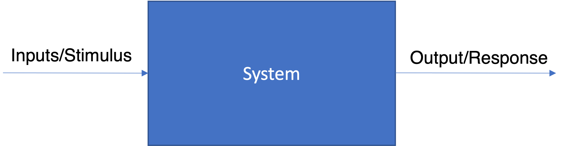
For example, our thermoregulatory system can take the ambient temperature as the input, and then decide to activate the sweat glands in our body, so as to maintain our core body temperature at a level suitable for our physiological processes. Then in the above diagram, the stimulus or input would have been the increase in ambient temperature while the output/response would have been the activation of the sweat glands.
The various systems within the human body vary vastly in size and function. Nevertheless, despite these differences, there must exist a way for these systems to communicate within their various subsystems as well as with the outside world. This is achieved using signals which encode information, typically by varying their "energy" content. Within the body, these are often called biosignals and the variation, specific energy fluctuations.
Table 1.1 of the textbook lists a few types of these.
| Energy | Variable Measured | Biosignal |
|---|---|---|
| Chemical | Chemical activity and/or concentration | Blood ions, O2, CO2, pH, hormonal concentrations, and other chemistry |
| Mechanical | Position, force, torque, or pressure | Muscle movement; Cardiovascular pressures, muscle contractility; Valve and other cardiac sounds |
| Electrical | Voltage, current | EEG, ECG, EMG, EOG, ERG, EGG, GSR |
| Thermal | Temperature | Body temperature, thermography |
Transducers & biotransducers
A device that is capable of converting between different types of energy is called transducer. Thus, generators and motors and piezoelectrics are all transducers. However, within the realm of signal processing, by a transducer we often mean a device that is used to convert information encoded using one form of energy, to another form. That is to say, the primary objective, of a biotransducer, is not energy conversion, but rather information processing. For example, a force sensor coupled with an EMG device might convert force exerted at the transducer to electrical energy, which allows for measuring the levels of force; say by way of voltage. However, both 0 N and 1000 N of force can get mapped to a 0 - 5V range, thus making the transducer a very inefficient energy conversion device. When making physiological measurements, by default all biosignals are converted to electrical signals for further processing using biotransducers.
Biotransducers are critical elements in systems because the accuracy and resolution of any measurement made on a physiological process depends on them. Typically, there are three strategies to make measurements from physiological systems.
A biotransducer is used to detect energy/signal generated within the body (thermometer, pulse-oximeter, etc.)
An external source of energy is used to turn the body into a signal source (PET, MRI, etc.)
An external signal source's variation is measured as it passes through the body (e.g., x-rays).
The table below lists a few biotransducers that convert physiological signals to electrical ones.
| Acronym | Full form | Organ involved |
|---|---|---|
| ECG | electrocardiogram | heart |
| EEG | electroencephalogram | brain |
| EMG | electromyogram | muscle |
| EOG | electrooculogram | eye |
| ERG | electroretinogram | retina |
| EGG | electrogastrogram | stomach |
Signal representation & encoding
Recall that signals encode information by way of variations in their energy content. Typically, for one-dimensional signals, these variations are captured in their amplitude and frequency. Thus, the same signal can be equivalently represented in the time domain or in the frequency domain (the subject of Chapter 3 and 4 in the textbook). However, since we are in the computer age, we first focus on the difference between continuous (also called analog) signals and discrete (also called digital) signals.[1]
Analog vs. Digital signals
Recall a signal may be mathematically represented as a mapping
from a domain to its range . The distinction between analog and digital signals lies in whether or , i.e. the real line or the integers.
For example, suppose a temperature transducer encodes room temperature into voltage as shown in the table below:
| Temperature (Celsius) | Voltage (Volts) |
|---|---|
| -10.0 | 0.0 |
| 0.0 | 5.0 |
| 10.0 | 10.0 |
| 20.0 | 15.0 |
Then the ensuing encoding equation for temperature in terms of voltage is:
It is clear that for this particular application and encoding scheme, and thus are continuous signals.
For use in a computer or digital applications, continuous signals must be converted into a series of numbers through a process called sampling.
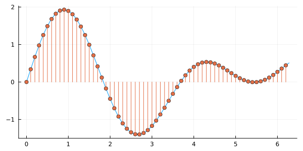
This typically involves partitioning the domain into equally sized intervals and recording the value of the signal at the end points of the constituent intervals. Then is called the sampling interval and the sequential numbers represent the discrete version of the analog signal . The sampling frequency is the reciprocal of .
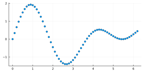
The above signal is a discrete version of the continuous signal and is represented in the computer by a sequence or array of numbers. To avoid specifying the domain of the argument of each time, it is convenient to adopt the notation for continuous signals and for digital signals. Note that, since computers can only represent digital signals, typically an analog-to-digital conversion also involves a partitioning of the range of as well.
The relationship between a continuous signal and its discrete counterpart is not an exact one; indeed the conditions necessary for the existence of a meaningful relationship between a continuous signal and its discrete version are described in Chapter 4.
(For now we will assume that all computer-based signals used in examples and problems are accurate representations of their associated continuous signals.)
Frequency domain vs. Time domain
As mentioned earlier, signals admit equivalent frequency and time domain representations. The time-domain graph shows how a signal changes over time, whereas a frequency-domain graph shows how much of the signal lies within each given frequency band over a range of frequencies. A complete frequency-domain representation also includes information on the phase shift that must be applied to sinusoids at each frequency in order to be able to recombine[2] the components and recover the original time signal.
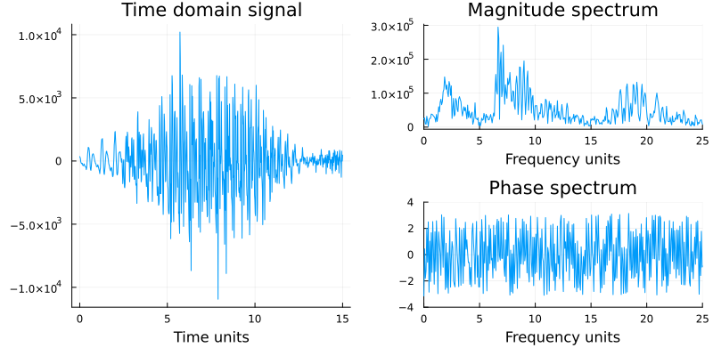
The figure above (c.f. Figure 1.7 from the textbook) shows an EEG time-domain signal (on the left) transformed into its magnitude and phase frequency-domain representations. The magnitude does show some interesting features: peaks around 1-3 Hz and 16-18 Hz, and a large peak around 7-8 Hz. These peaks in frequency are well known to neurologists.
In later lectures (corresponding to Chapters 3 and 4 in the textbook) we will learn techniques for moving between different types and representations of signals (time domain frequency domain and continuous time discrete time). The figure below summarizes these transformations.
Images as signals
Digital image signals are typically represented as two-dimensional (2D) arrays of discrete signal samples, commonly termed matrices[3]. Therefore, images can often be treated with the same mathematical analyses as signals although some techniques need to be specially extended to two dimensional data.
In most scientific programming languages, images are represented no different from normal numeric arrays. This means that standard mathematical operations can be applied to an image; conceptually the image is just another matrix to MATLAB/NumPy/Julia. The code below shows some basic mathematical and threshold operations applied to an MR image of the brain. Note that you will need to download the brain.mat file from the companion website to the textbook.
% Example 1.3  Example to apply some mathematical and threshold operations
%   to an MR image %  of the brain.

clear all; close all;
load brain;         		% Load image
subplot(2,2,1);             	% Display the images 2 by 2
pcolor(I);           		% Display original image
colormap(bone);             	% Grayscale color map
caxis([0 1]);        		% Fix pcolor scale
title('Orignal Image');

subplot(2,2,2);
I1 = I + .3;			% Brighten the image by adding 0.3
pcolor(I1);           		% Display original image
colormap(bone);             	% Grayscale color map
caxis([0 1]);        		% Fix pcolor scale
title('Lightened');

subplot(2,2,3);
I1 = 1.75*I;			% Increase image contrast by multiplying by 1.75
pcolor(I1);           		% Display new image
colormap(bone);             	% Grayscale color map
caxis([0 1]);        		% Fix pcolor scale
title('Contrast Enhansed');

subplot(2,2,4);
[r, c] = size(I);           	% Get image dimensions
thresh = 0.25;			% Set threshold
for k = 1:r
    for j = 1:c
        if I(k,j) < thresh 	% Test each pixel separately
            I1(k,j) = 1;	% If low make corresponding pixel white (1)
        else
            I1(k,j) = 0;	% Otherwise make it black (0)
        end
    end
end
pcolor(I1);           		% Display new image
colormap(bone);             	% Grayscale color map
caxis([0 1]);        		% Fix pcolor scale
title('Thresholded');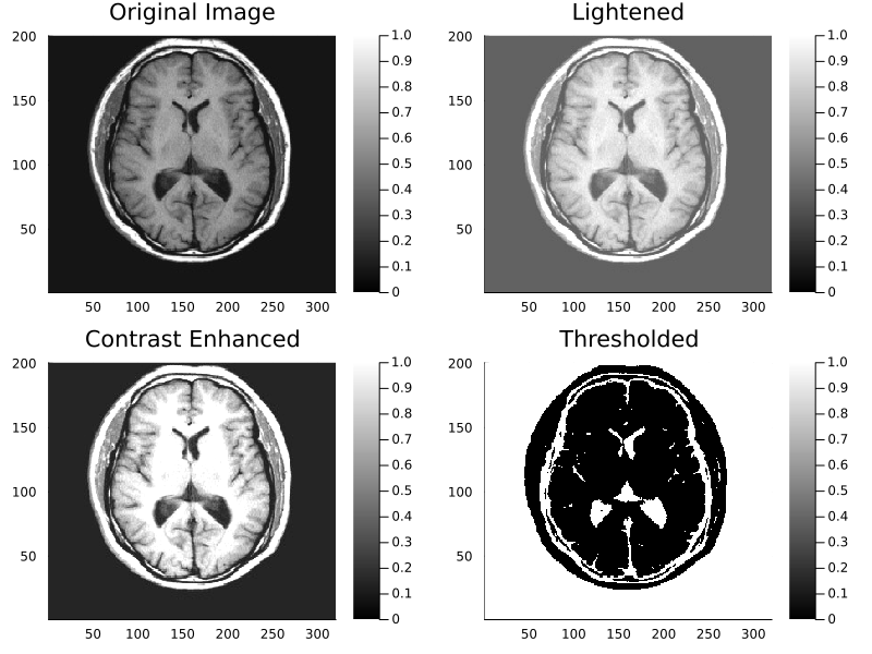
| [1] | The textbooks also makes a big distinction between 1-dimensional (time-series) and 2-dimensional signals (images), a convention which we will avoid because the time index (be it discrete or continuous) is almost always subsumed into the columns of a multi-dimensional signal for signal processing applications. |
| [2] | This is the essence of Fourier transforms as we will see in Chapter 3 of CSSB. |
| [3] | Strictly speaking, this is only true for grayscale images since color images are actually multidimensional arrays; i.e. matrices stacked together, one matrix per color channel (R-red, G-green, B-blue) |