ECE 486 Control Systems
Lecture 16
Bode’s Gain-Phase Relationship
Last time, we discussed stability in terms of frequency response. More specifically, we can tell how far we are from instability by identifying gain margin and phase margin on Bode plots.
In this lecture, we will study Bode’s Gain-Phase Relationship and use this as a guideline to design controllers using frequency response. We need to understand the effect of various types of controllers (PD/lead, PI/lag etc.) on the closed loop performance by reading the open loop Bode plot. Then we will develop frequency response techniques for shaping transient and steady state response using dynamic compensation.
Recall the unity feedback configuration as shown in Figure 1.

Figure 1: Unity feedback configuration with open loop transfer function \(KG(s)\)
Assuming that \(G(s)\) is minimum-phase, i.e., it has no Right Half Plane zeros, we derived in Lecture 14 the following for the Bode plot of \(KG(s)\)
| low freq. | real zero/pole | complex zero/pole | |
| mag. (slope) | \(n\) | up/down by \(1\) | up/down by \(2\) |
| phase | \(n \times 90^\circ\) | up/down by \(90^\circ\) | up/down by \(180^\circ\) |
We can state this succinctly as follows,
Gain-Phase Relationship: Far enough from breakpoints, \[ \text{Phase} \approx \text{Magnitude Slope} \times 90^\circ. \]
This suggests the following rule of thumb.
- If \(M\) has slope \(-2\) at \(\omega_c\), by the above Gain-Phase relation, we have \(\phi(\omega_c) = -180^\circ\), thus \(\color{red}{\text{no}}\) phase margin.
- If \(M\) has slope \(-1\) at \(\omega_c\), by the above Gain-Phase relation, we have \(\phi(\omega_c) = -90^\circ\), thus we have phase margin \(\color{blue}{{\rm PM} = 90^\circ}\).
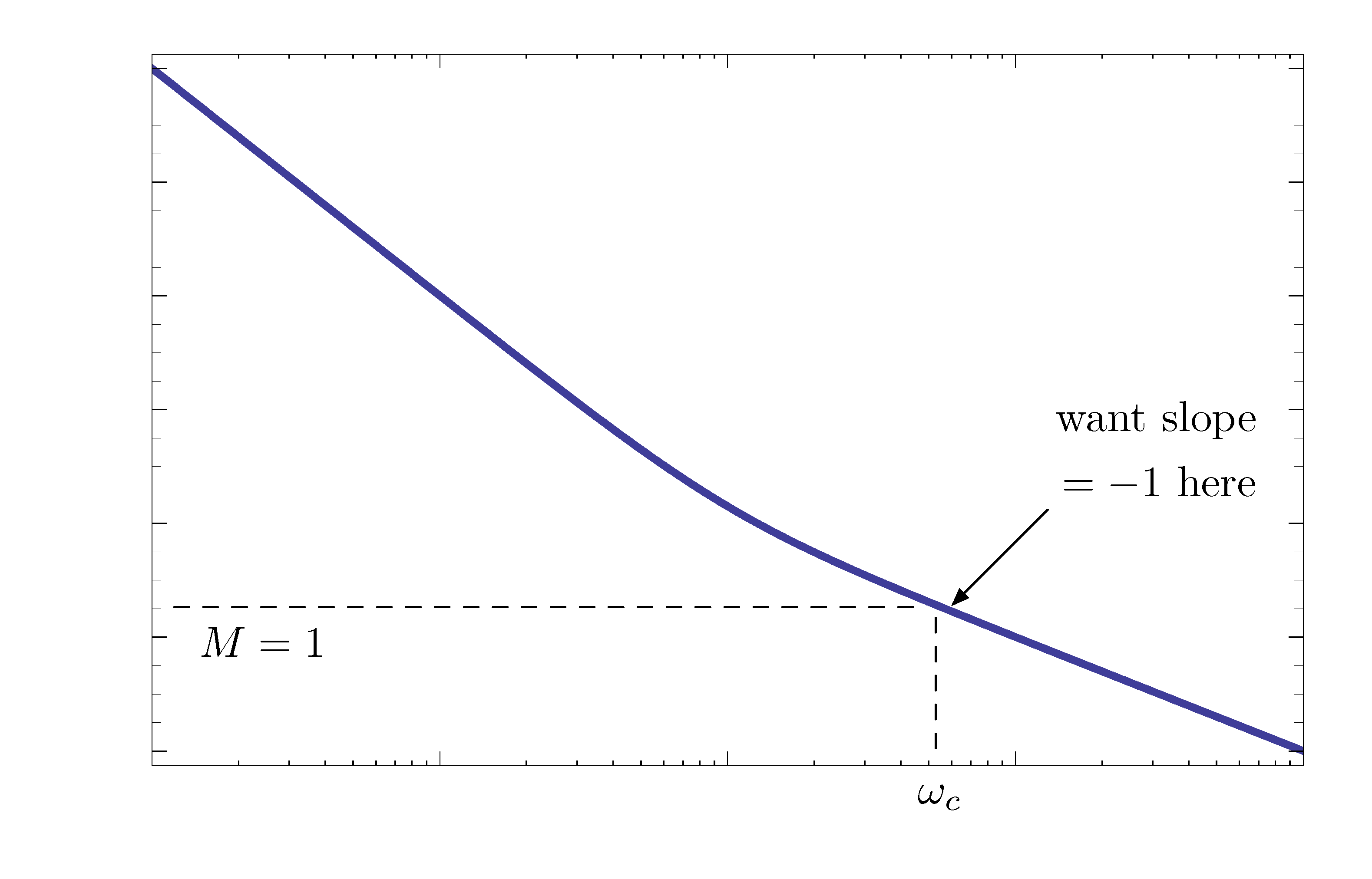
Figure 2: Gain-Phase relationship as design guideline
Other than what is shown in Figure 2, similar considerations may apply when magnitude plot has positive slopes depending on different transfer functions.
Gain-Phase Relationship and Bandwidth
By the design guideline above, when phase margin is \(90^\circ\),
\begin{align*} \begin{cases} |KG(j\omega_c)| &= 1 \\ \angle G(j\omega_c) &= -90^\circ \end{cases} \implies KG(j\omega_c) = -j. \end{align*}By the unity feedback configuration in Figure 1, we can evaluate the closed loop transfer function at \(s = j\omega_c\),
\begin{align*} T(j\omega_c) &= \frac{KG(j\omega_c)}{1+KG(j\omega_c)} \\ &= \frac{-j}{1-j}. \\ |T(j\omega_c)| &= \left|\frac{-j}{1-j}\right| \\ &= \frac{1}{\sqrt{2}}. \\ \tag{1} \label{d16_eq1} \implies \omega_c &= \omega_{\rm BW}. \text{ ($\omega_{\rm BW}$ is bandwidth)} \end{align*}Note though, \(|KG(j\omega)| \to \infty\) as \(\omega \to 0\) if it has a Type 1 factor \(\frac{K_0}{(j\omega)^n}\) as shown in its magnitude plot in Figure 2.
\begin{align*} |T(0)| &= \lim_{\omega \to 0} \frac{|KG(j\omega)|}{|1+KG(j\omega)|} \\ &= 1. \end{align*}Relationship between crossover frequency \(\omega_c\) and bandwidth \(\omega_{\rm BW}\):
- If \(\text{PM} = 90^\circ\), then \(\omega_c = \omega_{\rm BW}\).
- If \(\text{PM} < 90^\circ\), then \(\omega_c \le \omega_{\rm BW} \le 2\omega_c\). (See FPE.)
Control Design Using Frequency Response
Bode’s Gain-Phase Relationship suggests that we can shape the time response of the closed loop system by choosing \(K\) or, more generally, a dynamic controller \(KD(s)\) to tune the Phase Margin.
In particular, from the quantitative Gain-Phase Relationship, we have
\[ \text{Magnitude slope at } \omega_c = -1 \implies \text{Phase at } \omega_c \approx -90^\circ, \]
which gives us phase margin of \(90^\circ\) and consequently good damping.
Consider the following example. Let \(G(s) = \frac{1}{s^2}\), a double integrator with unity feedback as shown in Figure 3.

Figure 3: Example of design using frequency response
Our objective is to design a controller \(KD(s)\) where \(K\) is some scalar gain, such that
- closed loop stability is guaranteed;
- the system enjoys good damping (will make this more precise in a bit);
- the system bandwidth \(\omega_{\rm BW} \approx 0.5\). It is always a closed-loop characteristic.
Then our naive strategy following the above Bode’s Gain-Phase Relationship would be
- if we manage slope of \(-1\) in magnitude plot at \(\omega_c\), then phase margin \(\text{PM} = 90^\circ\). So it implies good damping;
- if \({\rm PM} = 90^\circ\), then \(\omega_c = \omega_{\rm BW}\). By Equation \eqref{d16_eq1}, we want \(\omega_c \approx 0.5\) by the specification.
Trials: First Attempt with P-Control
If we apply P-control, \(KD(s) = K\). Then
\[ D(s) = 1 \, \implies \, KD(s)G(s) = KG(s) = \dfrac{K}{s^2}. \]
The Bode plot Figure 4 shows \(=-2\) everywhere, so no phase margin.
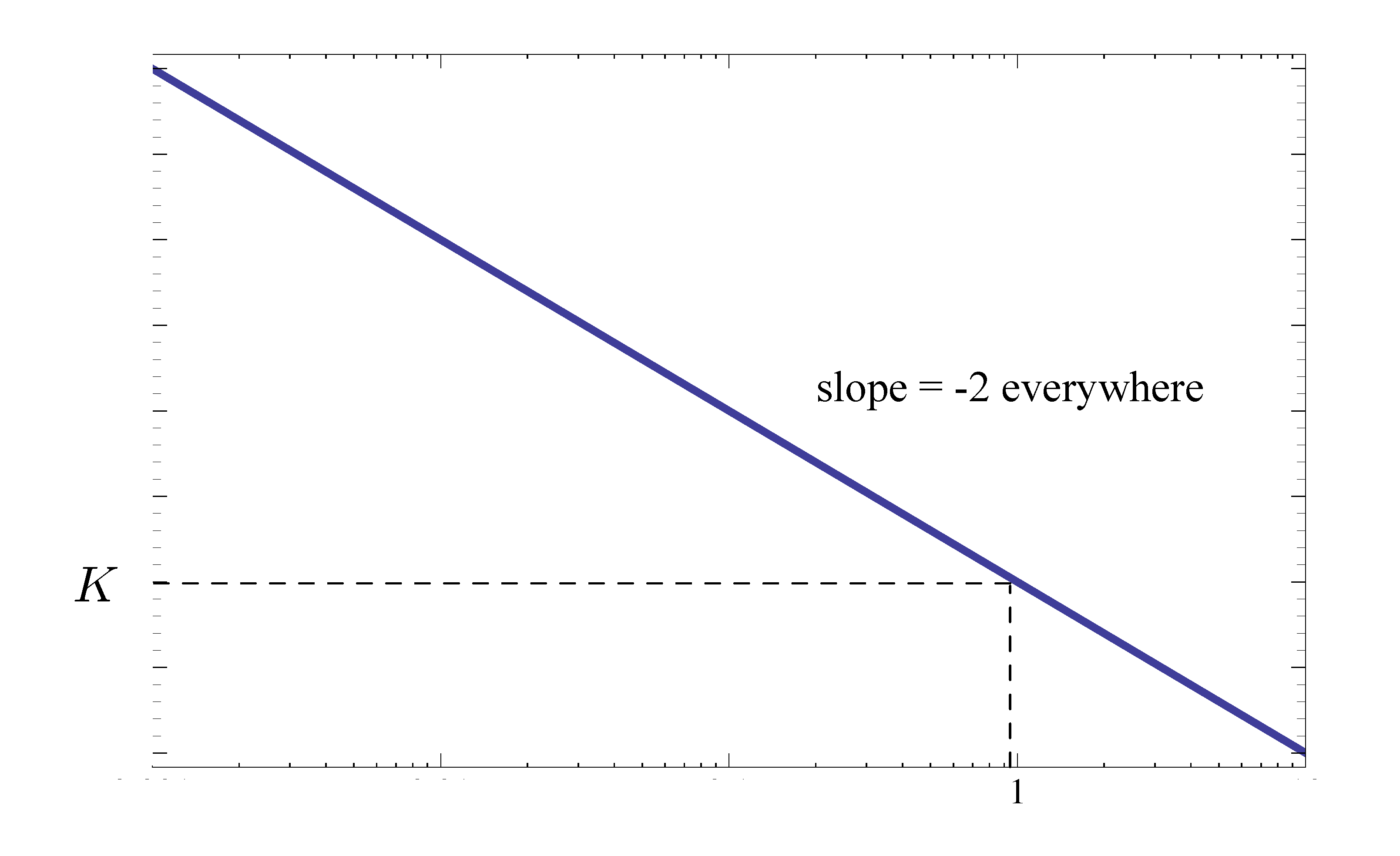
Figure 4: Bode plot for the first attempt with P-control
It confirms what we already knew; P-control alone would not do the job since if we calculate the characteristic equation explicitly,
\begin{align*} K+s^2 = 0, \end{align*}then the closed loop poles are on the imaginary axis, i.e., not strictly stable.
Trials: Second Attempt with PD-Control
Now let’s try PD-control with
\begin{align*} K D(s) &= K(\tau s + 1), \end{align*}where \(K_{\rm P} = K\), \(K_{\rm D} = K\tau\).
Then the open loop transfer function \(KD(s)G(s)\) becomes
\[KD(s)G(s) = \dfrac{K(\tau s + 1)}{s^2}.\]
Its Bode plot interpretation is that PD controller introduces a Type 2 factor in the numerator, which pushes the slope up by \(1\).
Compared to Figure 4 when \(D(s) = 1\), now PD-control has the effect of pushing the slope in magnitude plot of \(KD(s)G(s)\) from \(-2\) to \(-1\) past the breakpoint \(\omega = 1/\tau\).
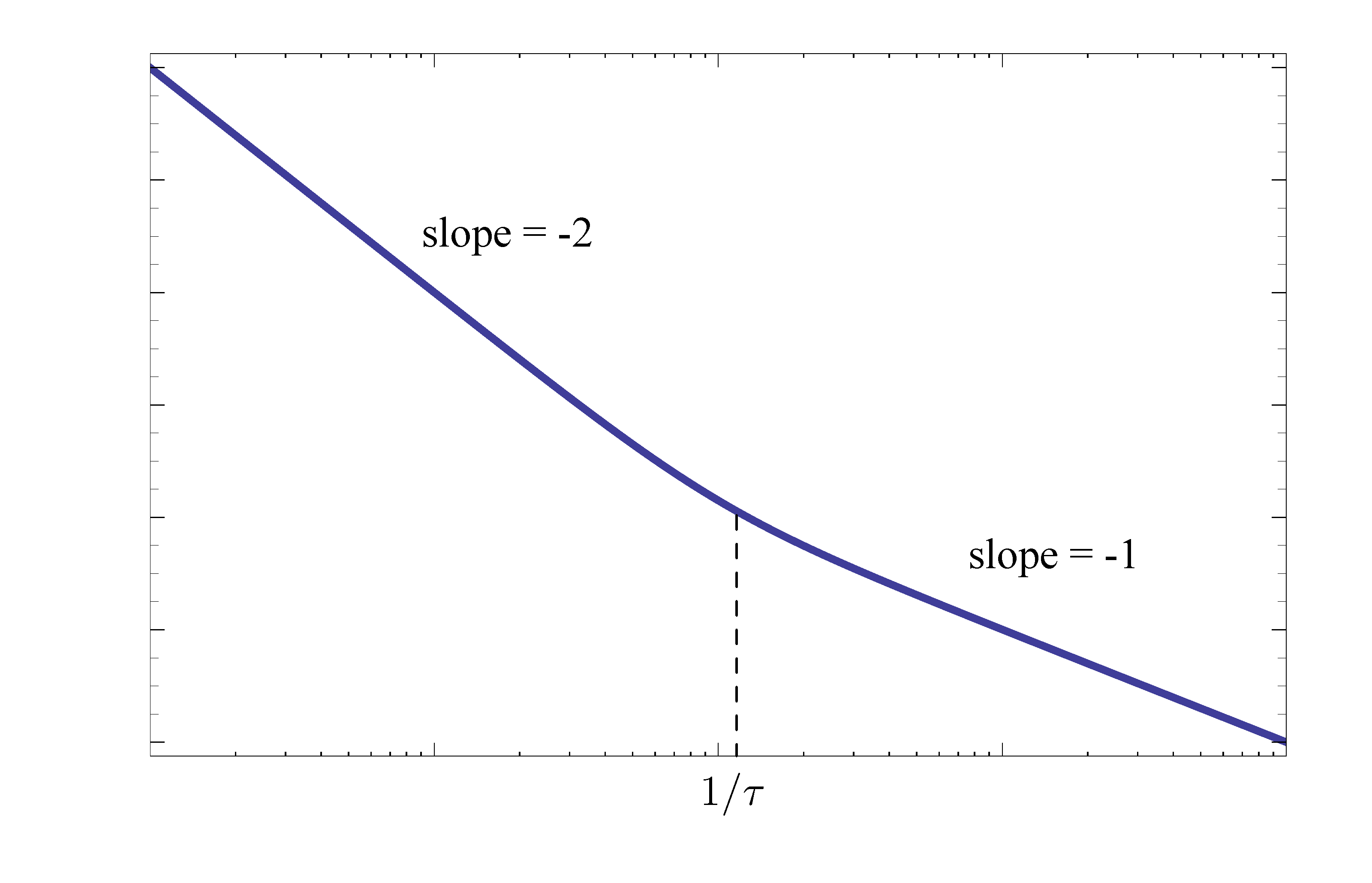
Figure 5: Bode plot for the second attempt with PD-control
For the Gain-Phase Relationship to be valid, choose the breakpoint several times smaller than desired \(\omega_c\). For example, let’s take \(\tau = 10\).
Then \(\dfrac{1}{\tau} = 0.1 = \dfrac{\omega_c}{5}\).
Now the open loop transfer function becomes
\[ KD(s)G(s) = \frac{K(10 s + 1)}{s^2}. \]
We want \(\omega_c \approx 0.5\), therefore
\begin{align*} M(j0.5) = 1 &\implies \left|KD(j0.5)G(j0.5)\right| = 1. \\ &\implies \frac{K |5j + 1|}{0.5^2} = 4K\sqrt{26} \approx 20K = 1. \\ &\implies K = \frac{1}{20}. \end{align*}Validation: Confirming Second Attempt with PD Control
With \(K = \frac{1}{20}\), our PD controller becomes
\[KD(s) = \dfrac{10s+1}{20}.\]
What have we accomplished with this controller?
- \({\rm PM} \approx 90^\circ\) at \(\omega_c = 0.5\).
- It still needs to be checked in Matlab and we need to iterate with different \(K\)’s if necessary.
Further we note several trade-offs here.
- We want \(\omega_{\rm BW}\) to be large enough for fast response, but not too large in order to avoid noise amplification at high frequencies. Recall the first half of the statement from Lecture 13 that larger \(\omega_{\rm BW} \iff\) larger \(\omega_n \iff\) smaller \(t_r\).
- PD control increases slope in magnitude plot \(\implies\) it increases \(\omega_c\) \(\implies\) it increases \(\omega_{\rm BW}\), hence faster response.
- But the usual caveat holds — D-control is not physically realizable, so we turn to its approximate lead compensation.
Lead Compensation in Bode Plot
We shall consider the lead controller in Equation \eqref{d16_eq2} momentarily and return to our example with lead control design thereafter.
\[\tag{2} \label{d16_eq2} KD(s) = K \frac{s+z}{s+p}, \, p \gg z. \]
Rewrite it in Bode form
\[ KD(s) = \frac{Kz \left(\frac{s}{z}+1\right)}{p \left(\frac{s}{p}+1\right)}. \]
Or, absorbing \(\frac{z}p\) into the overall gain, we have
\[ KD(s) = \dfrac{K\left(\frac{s}{z}+1\right)}{\left(\frac{s}{p}+1\right)}. \]
There are two breakpoints
- Type 2 factor with a zero has a breakpoint at \(\omega = z\). Note we hit this breakpoint frequency first since \(z \ll p\).
- Type 2 factor with a pole has a breakpoint at \(\omega = p\).
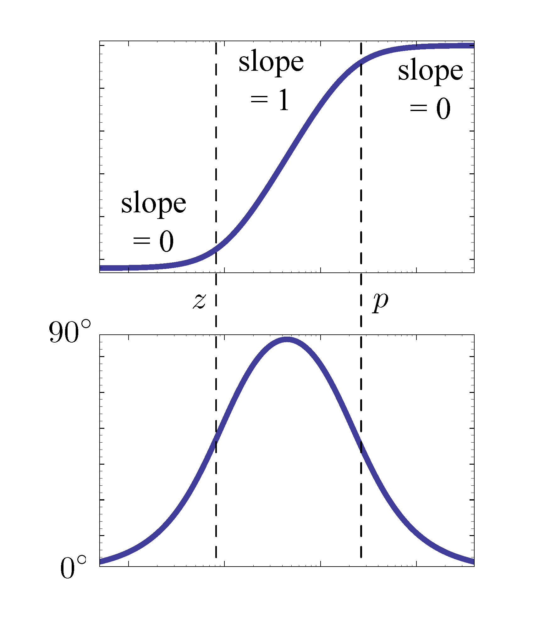
Figure 6: Bode plot for lead controller \(K\frac{s+z}{s+p}\)
Figure 6 shows the Bode plot for lead control in Equation \eqref{d16_eq2}.
We see
- the magnitude levels off at high frequencies, i.e., minor noise amplification;
- it can bump up phase for some frequencies, hence the term phase lead.
Next we will look into the relationship between lead compensation and phase margin.
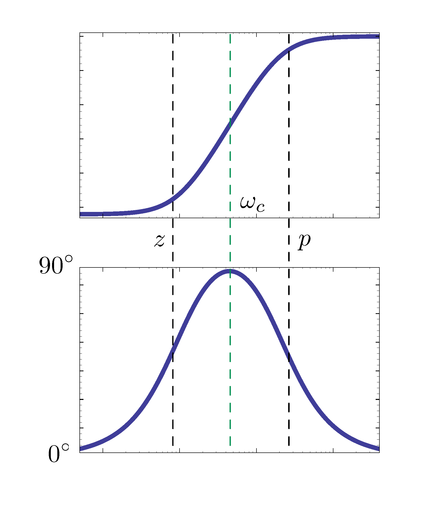
Figure 7: Bode plot for lead controller \(K\frac{s+z}{s+p}\) with \(\omega_c\) centered
As shown in Figure 7, for the best effect on phase margin, \(\omega_c\) should be halfway between \(z\) and \(p\) on the log scale plot. Therefore
\begin{align*} \log \omega_c &= \frac{\log z + \log p}{2}, \\ \text{or } \omega_c &= \sqrt{z p}. \end{align*}This means we align the crossover frequency with the geometric mean of \(z\) and \(p\).
By the phase plot in Figure 7, we want large difference \(p-z\) between \(z\) and \(p\) so that lead control can contribute a large phase bump which will be closer to \(90^\circ\).
But on the other hand it also means the “band” between \(z\) and \(p\) in the magnitude plot in Figure 7 becomes wider. It follows that it levels off only at larger frequencies, i.e., worse noise amplification.
Trials: Third Attempt with Lead Control
Now let’s return to our example of controlling \(G(s) = \frac{1}{s^2}\). This time we use lead compensation.
With lead control, the magnitude Bode plot of \(KD(s)G(s)\) shall look like Figure 8.
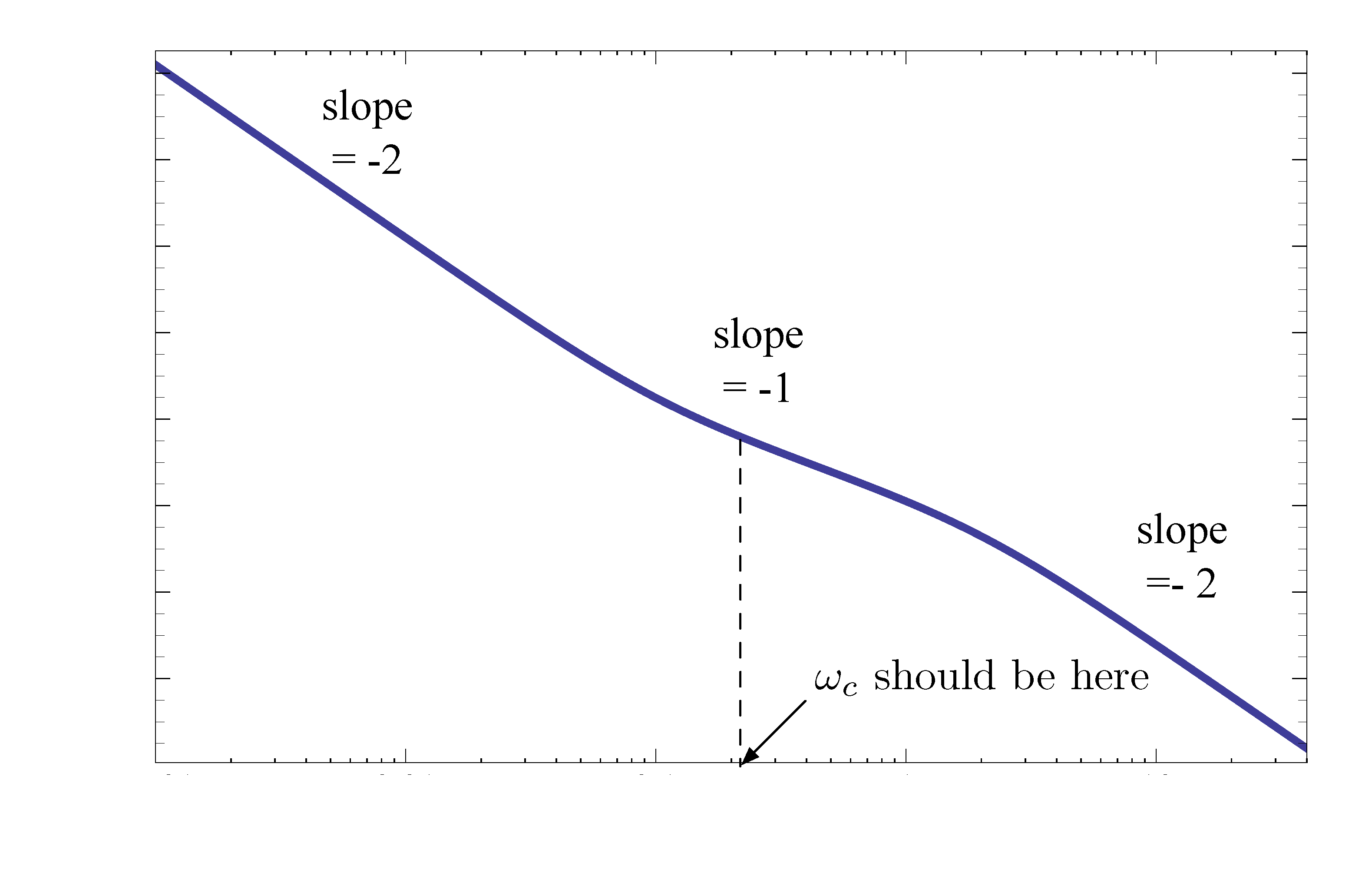
Figure 8: Bode plot for \(KD(s)G(s)\) with lead control
The lead controller raises the slope of magnitude plot for some frequencies thus adding a lead controller will increase \(\omega_c\).
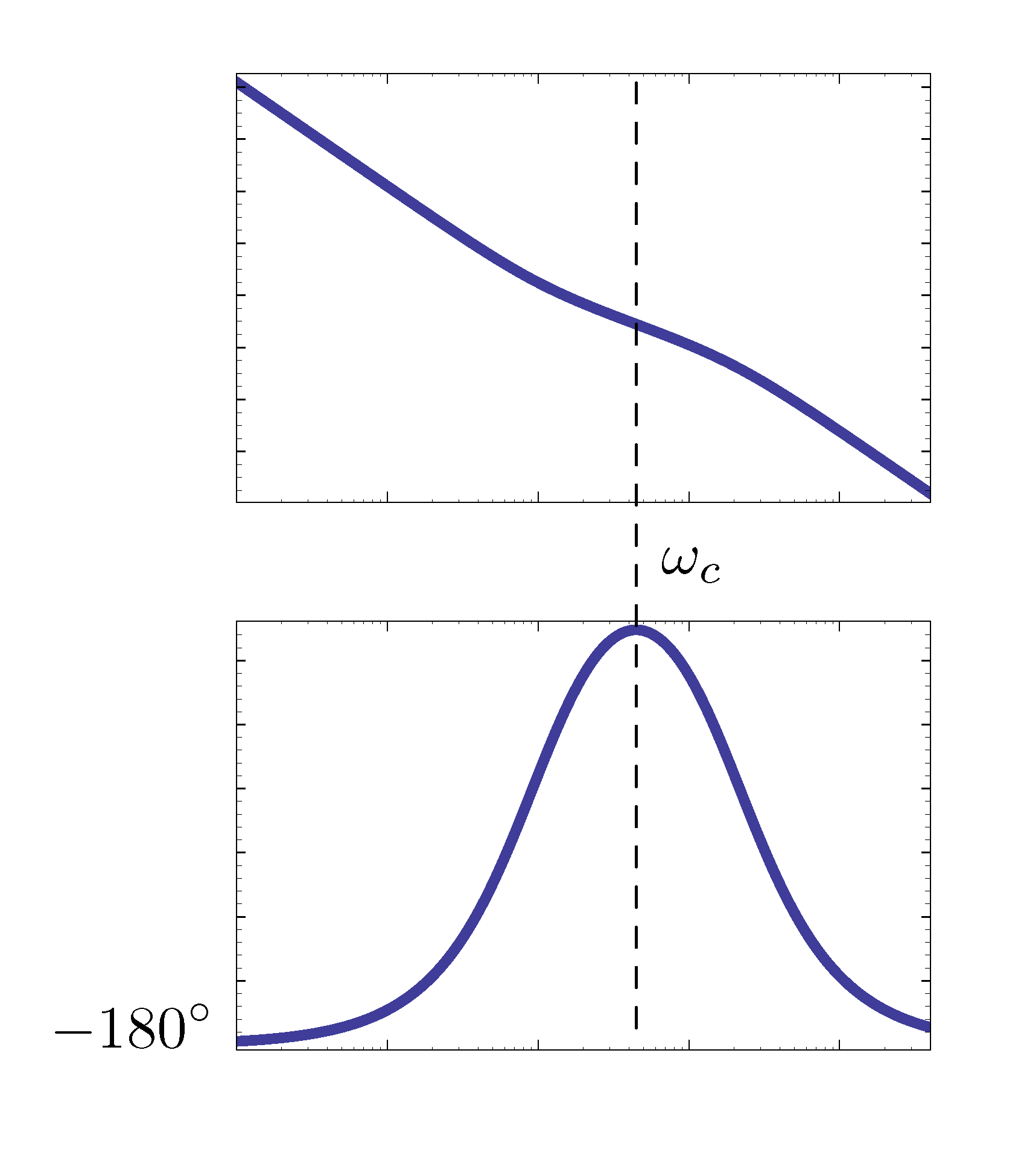
Figure 9: Bode plot for \(KD(s)G(s)\) with lead control
For example, with lead controller where \(K=1/4\),
- adding lead increases \(\omega_c\);
- phase margin \({\rm PM} < 90^\circ\);
- bandwidth \(\omega_{\rm BW}\) may be \(> \omega_c\).
To be on the safe side, we choose another \(K\) so that
\[ \omega_c = \frac{\omega_{\rm BW}}{2}. \]
Recall this is because generally \(\omega_c \le \omega_{\rm BW} \le 2\omega_c\).
Thus, we want
\[ \omega_c = 0.25 \implies K = \frac{1}{16}. \]
Next we pick \(z\) and \(p\) so that \(\omega_c\) is approximately their geometric mean, for example,
\begin{align*} & z=0.1,\, p=2. \\ & \sqrt{z \cdot p} = \sqrt{0.2} \approx 0.447. \end{align*}Then the resulting lead controller is
\begin{align*} KD(s) = \frac{1}{16} \frac{\dfrac{s}{0.1}+1}{\dfrac{s}{2}+1}. \end{align*}As an alternative, what we did in the lecture was
- Based on \(\omega_c = 0.25\) and \(\omega_c = \sqrt{zp}\), we obtained \(zp = \frac{1}{16}\).
- To be on the safer side, we let the gap between breakpoints \(z\) and \(p\) be wide enough so that crossover frequency \(\omega_c\) is not close to either of them. For example, set \(z = 0.01\) and \(p = 6.25\).
- Lastly, computed the \(K\) based on \(|KD(\omega_c)G(\omega_c)| = 1\).
It may still need to be refined using Matlab though.
To recap, control design using frequency response follows the general design procedure below.
- Choose a \(K\) to get desired bandwidth specifically without lead component \(\frac{s+z}{s+p}\).
- Choose a lead zero and a pole to get desired phase margin.
- In general, we should first check PM with \(K\) from 1, without lead, to see how much more PM bump we need.
- Check design and iterate until specs are met.
We shall bear in mind that this is an intuitive procedure; it’s not very precise. Sometimes it requires several rounds of trial and error.