ECE 486 Control Systems
Lecture 13
Lag Compensator (Continued)
Recall from last time, we introduced the lead and lag compensators and we began our investigation of approximating PI control via dynamic compensation by using a lag compensator. We shall continue this line of discussion.
Approximate PI via Dynamic Compensation
Recall from last time, a generic PI controller \(K_{\rm P} + \frac{K_{\rm I}}s\) can be approximated by a lag compensator, assuming \(z = \frac{ K_{\rm I} }{ K_{\rm P} }\),
\begin{align*} \text{replace }\, K \frac{s+z}{s} \quad \text{with} \quad K\frac{s+z}{s+p}, \text{ where $p < z$}. \end{align*}The replacement results in a lag compensator or a lag controller. Hence we use lag controllers as dynamic compensators for approximate PI control.
Consider an unstable plant \(G_p(s) = \frac{1}{s-1}\) with lag compensator \(G_c(s) = K \frac{s+z}{s+p}\), \(p < z\). Bear in mind that this lag compensator is used to approximate a PI controller which, as the nominal controller, has perfect tracking.
How good is this approximate PI controller, i.e., how good the lag compensator is in terms of tracking a constant reference?
To guarantee closed loop stability, there shall be no Right Half Plane poles for
\[\frac{E(s)}{R(s)} = \dfrac{1}{1+G_c(s)G_p(s)}.\]
Therefore we can use the characteristic polynomial
\begin{align*} (s+p)(s-1) + K(s+z) &= 0 \\ s^2 + (K+p-1)s + Kz-p &= 0 \end{align*}to get the range \(K > 1-p\) and \(Kz > p\) for closed loop stability.
With closed-loop stability, further apply the Final Value Theorem, then we have
\begin{align*} e(\infty) &= \frac{1}{1+G_c(s)G_p(s)}\Big|_{s=0} \\ &= \frac{1}{1 + K\frac{s+z}{(s+p)(s-1)}}\Big|_{s=0} \\ &= \frac{1}{1-\frac{Kz}{p}}. \tag{1} \label{d13_eq1} \end{align*}Though the steady-state error in Equation \eqref{d13_eq1} is not exactly \(0\), it could be close to zero (and negative) if \(\frac{Kz}{p}\) is large. Lag compensation does not give perfect tracking (indeed, it does not change system type), but we can get as good a tracking as we want by playing with \(K,z,p\). On the other hand, unlike PI, lag compensation gives a stable controller.
Effect of Lag Compensation on Root Locus
Now consider
\[ L(s) = \frac{s+1}{(s+p)(s-1)} \]
in the case of PI control for unstable plant \(G_p (s) = \frac{1}{s - 1}\), where \(\frac{K_{\rm I}}{K_{\rm P}} = 1\) from last time.
By choosing a small \(p\) that is very close to zero, we can make the root locus arbitrarily close to PI root locus (given it is stable for large enough \(K\)). Indeed, say, try \(p=0.1\),
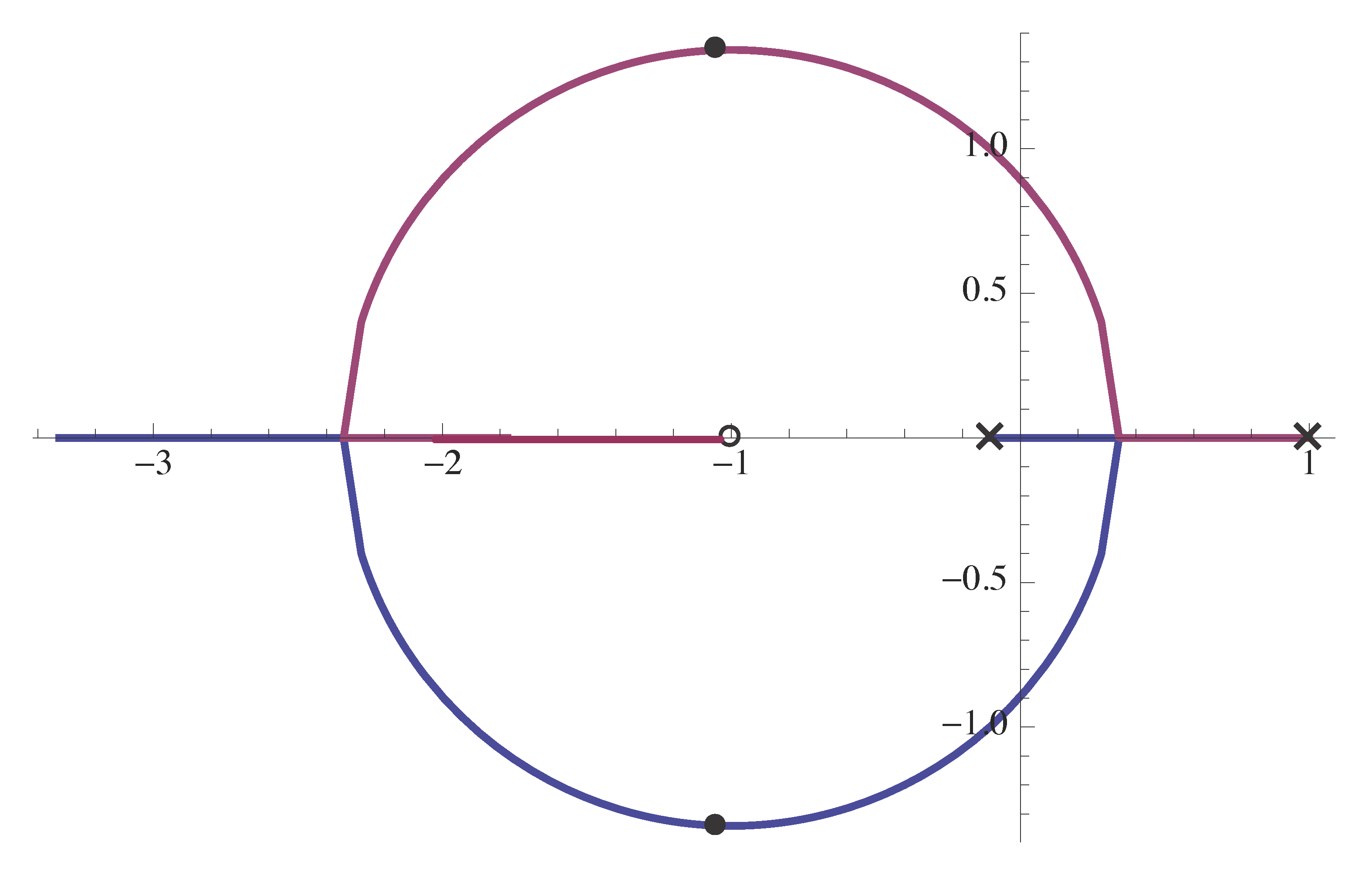
Figure 1: Root locus of using lag compensator to approximate PI control, \(p = 0.1\)
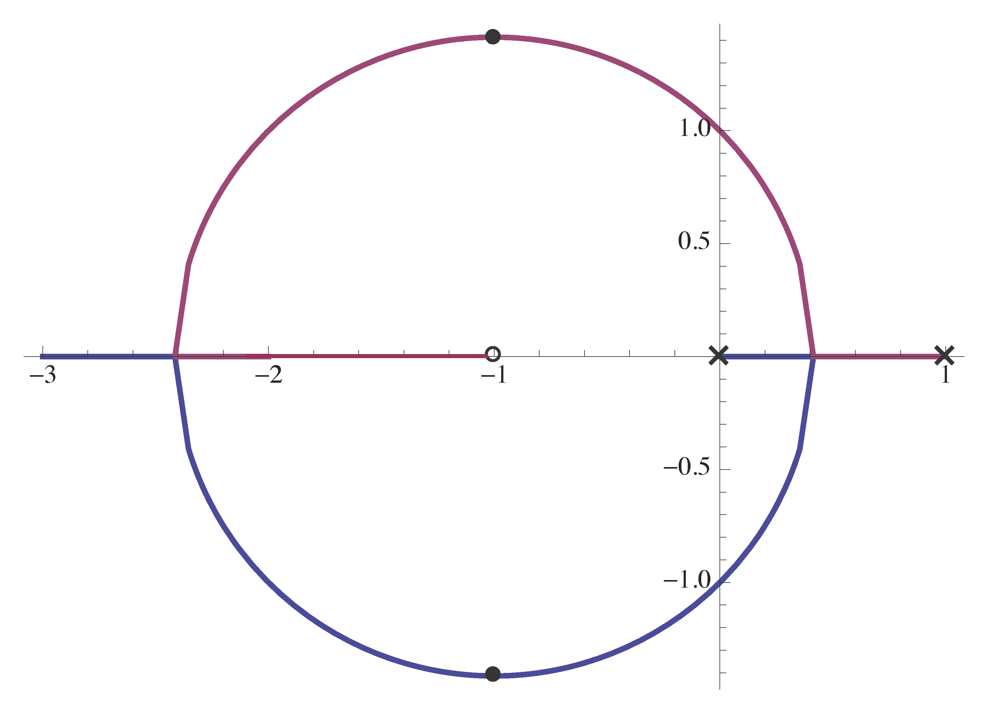
Figure 2: Root locus of using original PI control
Recall Figure 3 from last time, when we approximated PD control with a lead compensator \(K \frac{s + z}{s + p}\) with large \(p\), the root locus only resembles part of the original locus because the approximation
\[ s \mapsto \frac{ps}{s + p}, ~\, p \text{ large } \]
differs from the original by an extra pole. Here PI root locus versus lag control comparing to PD root locus versus lead control, there is no qualitative change in the shape of root locus, since we are not changing the number of poles or zeros of the original by using approximation
\[ \frac{1}s \mapsto \frac{1}{s + p}, ~\, p \text{ small}. \]
More Pole Placement Using Root locus
As before, we can choose \(z_{\rm lag}\) for a fixed \(p_{\rm lag}\) (or vice versa) based on desired pole locations.
The procedure is exactly the same as the one we used with lead control. In fact, depending on the pole locations, we may end up with either lead or lag.
We select parameters to satisfy the phase condition, i.e., points on root locus must always be such that \(\angle L(s) = 180^\circ\). One caveat though, if it turns out the following technique ends up with no sensible solutions, that means it may not be possible to have a lag compensator with specified pole locations.
Example: Again, consider the example with plant \(G_p(s)\) and controller \(G_c(s)\)
\[ G_p(s) = \dfrac{1}{s-1}, \qquad G_c(s) = K\dfrac{s+z}{s+p}. \]
Given \(p=2\), find \(K\) and \(z\) to place poles at \(-2 \pm 3j\).
Solution: The desired characteristic polynomial is given by
\begin{align*} (s+2)^2 + 9 = s^2 + 4s + 13. \end{align*}The damping ratio \(\zeta = \frac{2}{\sqrt{13}} \approx 0.555\).
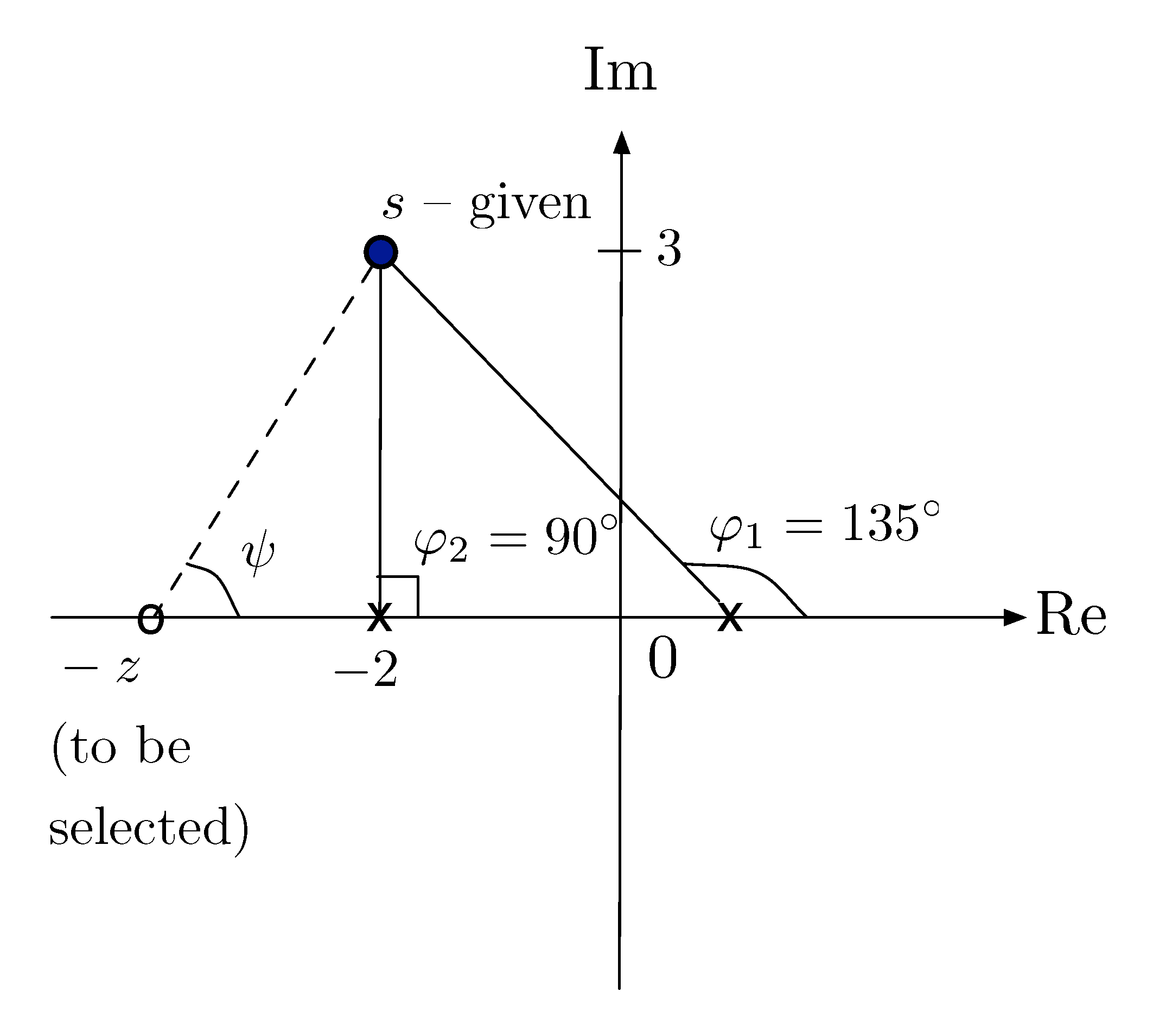
Figure 3: Find \(z\) by testing phase condition with given poles
Then we must have
\begin{align*} \underbrace{\psi}_{\text{angle from}\atop\text{$s$ to zero}} - \sum_i \underbrace{\varphi_i}_{\text{angles from}\atop\text{$s$ to poles}} = 180^\circ,& \\ \implies \psi = 180^\circ + \sum_i \varphi_i&. \end{align*}Based on the given pole locations, we already have \(\varphi_1 = 135^\circ\), \(\varphi_2 = 90^\circ\). Therefore
\begin{align*} \psi &= 180^\circ + \sum_i \varphi_i \\ &= 180^\circ + 135^\circ + 90^\circ \\ &= 405^\circ \\ &= 45^\circ \bmod 360^\circ. \end{align*}So we shall choose zero \(-z = -5\) as in Figure 4.
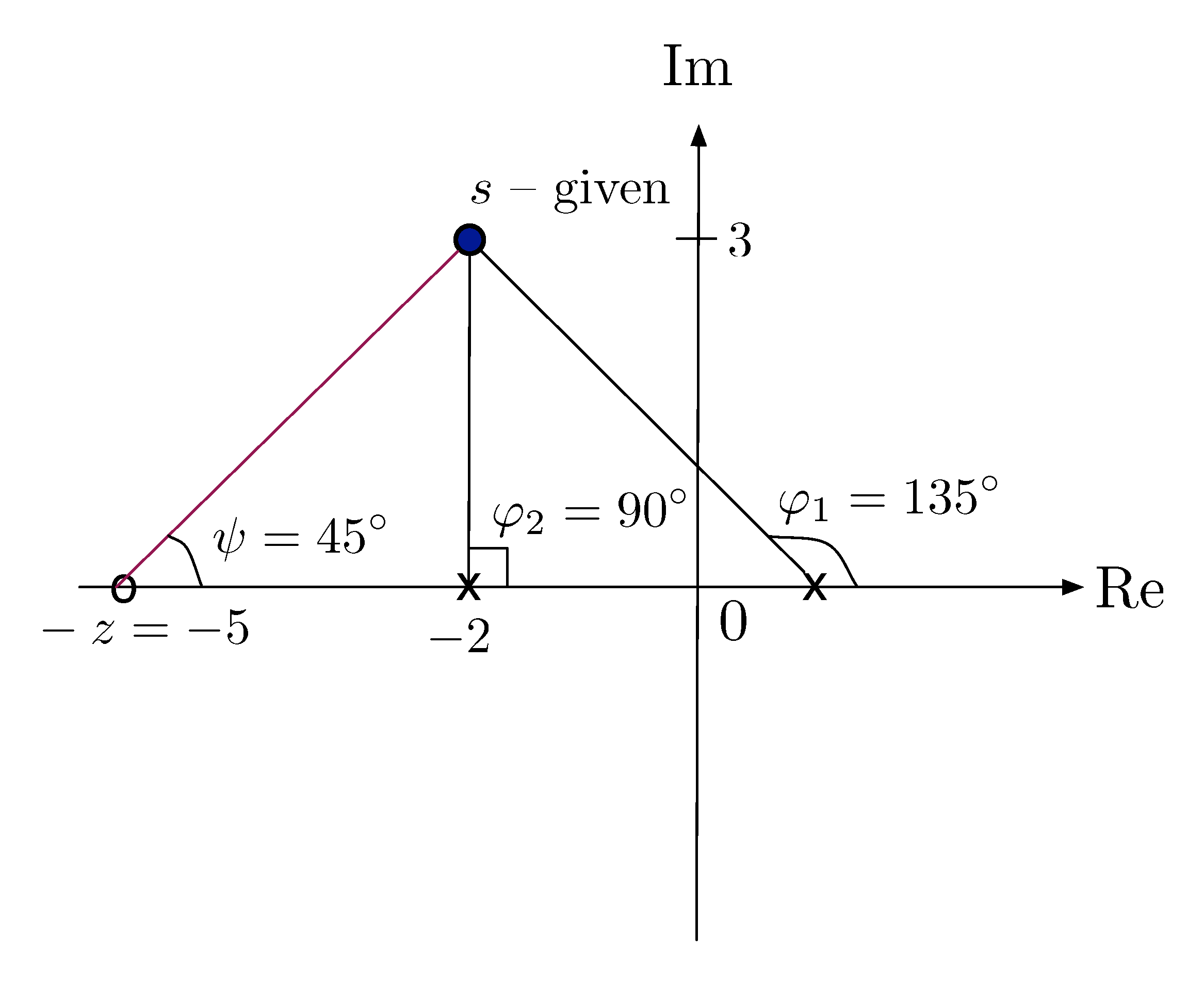
Figure 4: Find \(-z = -5\) with \(\psi = 45^\circ\)
With \(z = 5\), the resulting characteristic polynomial based on \(G_p(s) = \frac{1}{s - 1}\) and \(G_c(s) = K \frac{s + z}{s + p}\), is
\begin{align*} (s-1)(s+p) &+ K(s+z) \\ (s-1)(s+2) &+ K(s+5) \qquad \text{(by $p = 2$ given, $z = 5$ identified)} \\ s^2 + (K+1)s &+ 5K-2. \end{align*}Matching the desired characteristic polynomial from above
\begin{align*} s^2 + 4s + 13 &= s^2 + (K+1)s + 5K-2 \\ \implies K+1 &= 4, 5K-2 = 13. \end{align*}We can solve for \(K=3\).
Further by Equation \eqref{d13_eq1}, the steady state tracking error \(\left|\dfrac{1}{1-\frac{Kz}{p}}\right| = \dfrac{1}{6.5} \approx 15\%\).
So summarize what we have learned so far about PD control and PI control,
- PD control
- provides stability, allows us to shape transient response specs;
- replaces noncausal D-controller \(Ks\) with a causal, stable lead controller \(K \dfrac{s+z}{s+p}\), where \(p > z\);
- introduces a zero in Left Half Plane at \(-z\), hence pulls the root locus into LHP; but the shape of root locus differs depending on how large \(p\) is.
- PI control
- provides stability and perfect steady-state tracking of constant references;
- replaces unstable I-controller \(\frac{K}s\) with a stable lag controller \(K \dfrac{s+z}{s+p}\), where \(p < z\); and this does not change the shape of root locus compared to PI.
Therefore by combining PD and PI control, or their approximates lead and lag compensation, PID control can have features from both.
We will develop this further in homework and later in the course using frequency-response design methods. This is a new framework.
Frequency-Response Design Method
Recall the frequency response formula from Lecture 3,

Figure 5: Sinusoidal input and frequency response
\(M = M(\omega) = |G(j\omega)|\) and \(\phi = \phi(\omega) = \angle G(j\omega)\)
Also recall how this was derived,
- Using input \(u(t) = e^{st}\) for fixed \(s \in \CC\), the transfer function \(G(s)\) gives response \(y(t) = G(s)e^{st}\);
- Relate complex sine function to exponential by Euler’s formula, \(\sin(\omega t) = \frac{e^{j\omega t} - e^{-j\omega t}}{2j}\);
Then by linearity, the resulting response due to \(\sin (\omega t)\) is
\begin{align*} & \frac{G(j\omega) e^{j\omega t} - G(-j\omega)e^{-j\omega t}}{2j} \\ =& \frac{M(\omega)e^{j(\omega t + \phi(\omega))} - M(\omega)e^{-j(\omega t + \phi(\omega))}}{2j} \\ =& M(\omega) \sin(\omega t + \phi(\omega)), \end{align*}where \(G(j\omega) = M(\omega) e^{j\phi(\omega)}\).
As an example, for the prototype second order transfer function
\[ G(s) = \frac{\omega^2_n}{s^2 + 2\zeta\omega_n s + \omega^2_n}, \]
we have
\begin{align*} M(\omega) &= |G(j\omega)| \\ &= \left| \frac{\omega^2_n}{-\omega^2 + 2j\zeta\omega_n \omega + \omega^2_n}\right| \\ &= \left| \frac{1}{1 - \big(\frac{\omega}{\omega_n}\big)^2 + 2\zeta \frac{\omega}{\omega_n}j} \right| \\ &= \frac{1}{\sqrt{\left[1-\big(\frac{\omega}{\omega_n}\big)^2\right]^2 + 4\zeta^2\big(\frac{\omega}{\omega_n}\big)^2}} \tag{2} \label{d13_eq2}\\ &= \frac{1}{\sqrt{1 + (4\zeta^2-2)\big(\frac{\omega}{\omega_n}\big)^2 + \big(\frac{\omega}{\omega_n}\big)^4}}. \end{align*}We can plot \(M(\omega)\) as a function of \(\frac{\omega}{\omega_n}\) with various damping \(\zeta\) values as shown in Figure 6.
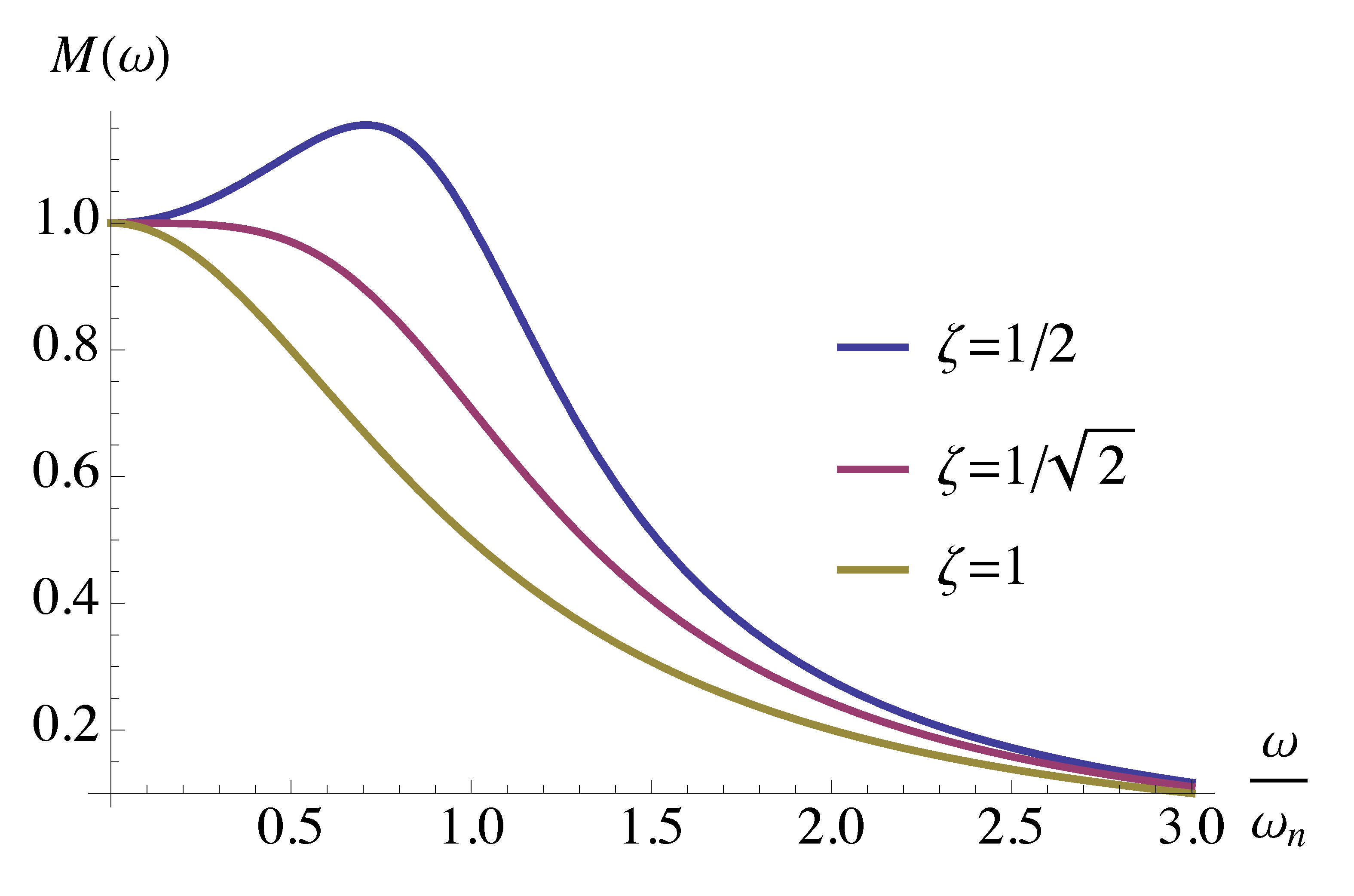
Figure 6: Magnitude \(M(\omega)\) as a function of \(\frac{\omega}{\omega_n}\)
Frequency Response Parameters
Here is a typical frequency response magnitude plot.
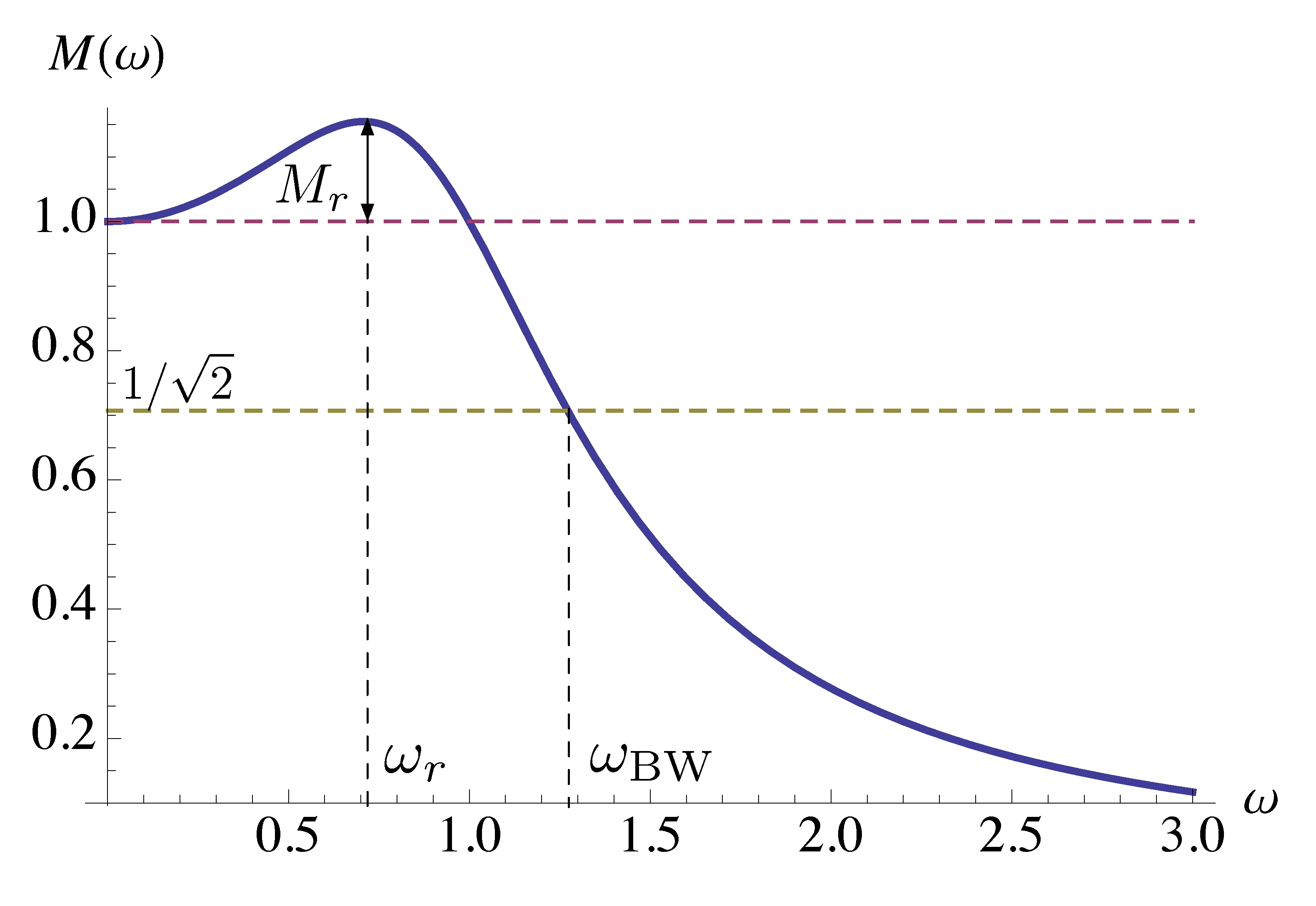
Figure 7: Typical frequency response magnitude plot
In Figure 7, \(\omega_r\) is called resonant frequency, \(M_r\) resonant peak and \(\omega_{\rm BW}\) bandwidth.
We can get the following formulas using calculus for Equation \eqref{d13_eq2}
\begin{align*} \omega_r &= \omega_n \sqrt{1-2\zeta^2} \\ M_r &= \dfrac{1}{2\zeta\sqrt{1-\zeta^2}}-1 \\ \omega_{\rm BW} &= \omega_n \underbrace{\sqrt{(1-2\zeta^2) + \sqrt{(1-2\zeta^2)^2+1}}}_{=1 \text{ for } \zeta = 1/\sqrt{2}}. \end{align*}Resonance formulas are valid for \(\zeta < \dfrac{1}{\sqrt{2}}\) for obvious reasons. If \(\zeta \ge \dfrac{1}{\sqrt{2}}\), then \(\omega_r = 0\), meaning no resonance.
If we know \(\omega_r, M_r, \omega_{\rm BW}\), we can determine \(\omega_n,\zeta\) and hence the time-domain specifications \(t_r,M_p,t_s\) etc.
Therefore all information about time response is also encoded in frequency response.
Frequency Response and Time-Domain Specs:
\begin{align*} \text{small $M_r$ } &\iff \text{ better damping} \\ \text{large $\omega_{\rm BW}$ } &\iff \text{ large $\omega_n$ } \iff \text{ smaller $t_r$} \end{align*}
Figure 8: Unity feedback configuration
The main idea of frequency response design method can be characterized by the following two step procedure
- Plot the frequency response of the open loop transfer function \(KG(s)\) or, more generally, \(D(s)G(s)\) at \(s=j\omega\);
- See how to relate this open loop frequency response to closed loop behavior.
We will work with two types of plots for \(KG(j\omega)\)
- Bode plots: magnitude \(|KG(j\omega)|\) and phase \(\angle KG(j\omega)\) versus frequency \(\omega\). You may have seen Bode plots before, e.g., in ECE 342.
- Nyquist plots: \({\rm Im} \big(KG(j\omega)\big)\) versus \({\rm Re}\big(KG(j\omega)\big)\), complex trajectories in $s$-plane as \(\omega\) ranges from \(-\infty\) to \(+\infty\).
Note on the Scale
Horizontal (\(\omega\)) Axis
We will use logarithmic scale with base \(10\) in order to display a wide range of frequencies.
We still mark the values of \(\omega\), not \(\log_{10}\omega\) on the horizontal axis, but the scale will be logarithmic as shown in Figure 9.

Figure 9: \(\omega\) axis in \(\log\) scale
Therefore, equal intervals on log scale correspond to decades in frequency.
Vertical Axis on Magnitude Plots
We will also use logarithmic scale, just as the frequency axis. The reason is by taking logarithm, we can convert multiplication to addition
\begin{align*} & |(M_1 e^{j\phi_1}) (M_2 e^{j\phi_2}) | = M_1 \cdot M_2 \\ & \log (M_1 M_2) = \log M_1 + \log M_2. \end{align*}This means that we can simply add the graphs of \(\log M_1(\omega)\) and \(\log M_2(\omega)\) to obtain the graph of \(\log \big(M_1(\omega)M_2(\omega)\big)\). The specific \(\log\) scale in use is Decibel scale.
\[ (M)_{\rm dB} = 20 \log_{10} M \text{, one decade $= 20\, {\rm dB}$}. \]
The number \(20\) in decibel is related to power.
Vertical Axis on Phase Plots
We will plot the phase on the usual linear scale. The reason is by De Moivre’s formula, the argument of product of two complex numbers is already the sum of arguments,
\begin{align*} \angle \left((M_1 e^{j\phi_1}) (M_2 e^{j\phi_2})\right) &= \angle \left( M_1M_2 e^{j(\phi_1 + \phi_2)}\right) \\ &= \phi_1 + \phi_2. \end{align*}This means that we can simply add the phase plots for two transfer functions to obtain the phase plot for their product.
| magnitude plot | phase plot | |
| horizontal scale | \(\log\) | \(\log\) |
| vertical scale | \(\log\) | linear |
We will learn to draw Bode plots by starting with simple factors and then building up to general transfer functions by considering products of these simple factors.