Lecture 08
Reading material: Examples in Chapter 3 of CSSB.
Now that in previous lectures we have discussed the Fourier transforms, and seen some examples of it analytically, in this lecture let us look at implementations of the same on software.
Reconstructing a wave from its Fourier expansion
Square wave
Let us consider the square wave from the beginning of Lecture 07. We derived that its Fourier coefficients were:
which were associated with the complex exponentials . Let us use this information to try and reconstruct the signal. As we have discussed previously, the square wave requires an infinite summation for its analytical expansion in terms of the Fourier coefficients. Since on a computer we do not have infinite memory, our approach will be to symmetrically truncate the summation in the reconstruction.
Let us start by writing three functions.
The first,
spool, is to collate together positive odd numbers up to and negative odd numbers up to .The second function will be to return the Fourier coefficient in the above equation.
The last function will be to evaluate the -th term in the expansion over the time variable . Here they are:
spool(N) = flatten([-1:-2:-N, 1:2:N])
F(k) = 2/(k*π*im)
kth_term(t) = k -> F(k) * exp.(2π*k*im*t)
Next we define N to use in the spool function above, the time variable on the interval . After that we evaluate the sum and extract only its real part (since the signal was real to begin with). The final command just plots the reconstruction.
N, t = 20, 0:0.01:5
y = real(sum(kth_term(t).(spool(N))))
title = "Reconstructed sq. wave for N=$N"
plot(t, y, label=false, title=title)
That really is it, six lines. Here is the whole code and the output:
using Plots, Base.Iterators

spool(N) = flatten([-1:-2:-N, 1:2:N])
F(k) = 2/(k*π*im)
kth_term(t) = k -> F(k) * exp.(2π*k*im*t)

N, t = 20, 0:0.01:5
y = real(sum(kth_term(t).(spool(N))))
title = "Reconstructed sq. wave for N=$N"
plot(t, y, label=false, title=title)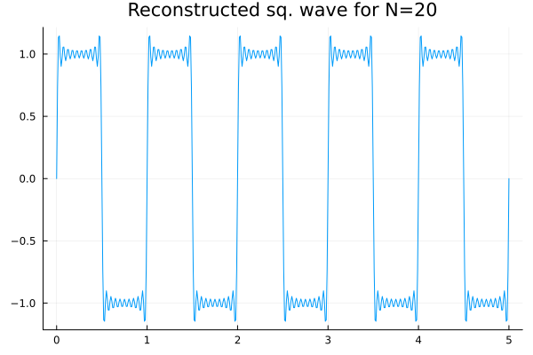
MATLAB Version
N = 20
t = 0:0.01:5
y = zeros(size(t))
sum_indices = [[-1:-2:-N], [1:2:N]]

for i=1:length(sum_indices)
	k = sum_indices(i)
	y = y + kth_term(k, t);
end

plot(t, real(y));

function y = kth_term(k, t)
	y = 2/(k*pi*1i)* exp(2*pi*k*1i.*t);
end
How about we try another one?
Triangle wave
Recall from the previous lecture note that we derived that the Fourier coefficients for the triangle wave as:
Following a similar strategy as last time we get that the following code and output recreate the triangle wave with as little as 10 terms in the sum.
using Plots, Base.Iterators

spool(N) = flatten([-1:-2:-N, 1:2:N])
a(k) = (4*sin(π*k/2)^2)/(k^2*π^2)
kth_term(t) = k -> a(k)*cos.(2π*k*t)

N, t = 10, 0:0.01:5
y = real(sum(kth_term(t).(spool(N))))
title = "Reconstructed △ wave for N=$N"
plot(t, y, label=false, title=title)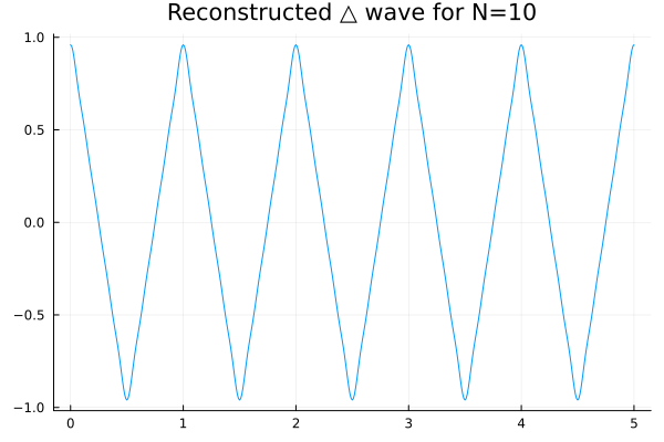
Example from CSSB
In Example 3.4 of CSSB we are shown a periodic waveform in Figure 3.13.They derive the complex Fourier coefficients in that case as:
Let us try to reconstruct the waveform using these:
using Plots

spool(N) = -N:1:N
C(k) = (exp(24//10)-1)/(24//10 -im*2π*k)
kth_term(t) = k -> C(k) * exp.(2π*k*im*t)

N, t = 50, 0:0.01:5
y = sum(kth_term(t).(spool(N)))
plot(t, real(y), label=false, title="Reconstructed wave for N=$N")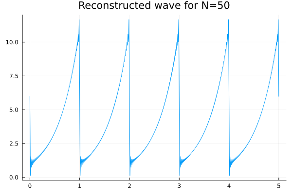
Computing the Fourier Transform
Now that we know how to reconstruct signals - i.e. to implement the synthesis equations in software, we should think of what tools we have at our disposal to implement the analysis equations.
Multiple examples in CSSB implement the analysis equations in great detail using MATLAB. Therefore, this lecture note will not focus on those; rather we will focus on examples of using MATLAB's fft function.
MATLAB's fft
Most open source languages ship with a version of the FFTW library while MATLAB ships with its on internally optimized version based on the FFTW library. In this class our inputs to fft are vectors. But this need not be the case. If you check the documentation you will find that you can pass multi-dimensional arrays to fft as well. The documentation tells us that in such a case, MATLAB prefers to treat N-D arrays as vectors along some dimension and then apply DFT to those vectors. This is different from vanilla and most other fftw which will perform DFT along all dimensions by default. The MATLAB equivalent for this is the fftn function. Apart from this difference, most of the behavior of the two functions is same.
If x is a real or complex vector then MATLAB's fft(x) returns a complex vector of the same size as x. You might think this odd for real valued vectors x because inherently has twice the dimension compared to , and so somehow the information doubled. This isn't true because if x is real then the DFT will have components that are complex conjugates of each other and so some information is redundant (in fact, exactly half the information).
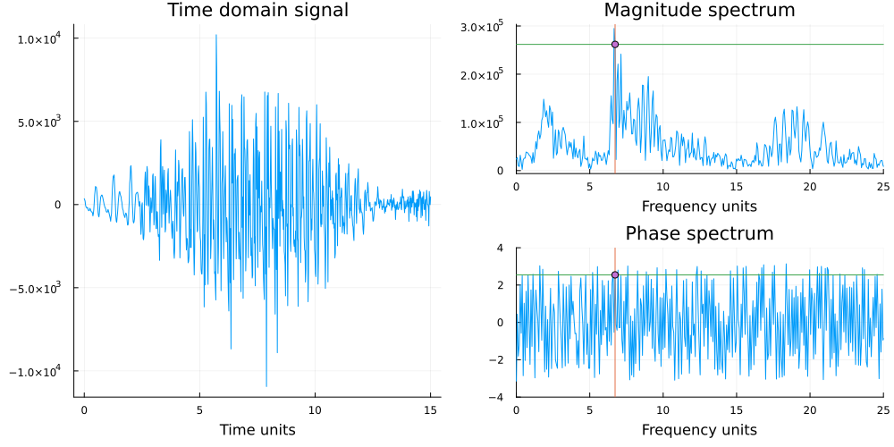
In each element of the complex valued output vector we get, there are three items of interest to us: (a) the magnitude and (b) the phase and (c) the frequency at which the previous two are applicable. Remember the example of the frequency domain representation that we have seen in multiple lectures past (shown below).
The output from the fft algorithm though, just returns a complex vector in Cartesian form. From this vector is straightforward enough to extract the phase (using the angle function) and the magnitude (using the abs) function. However, we don't have any information on the frequency vector, needed to generate a plot like the above.
Both in MATLAB's documentation as well as the examples in CSSB, this frequency vector is crafted by hand using information about the length of the vector input x and the sampling frequency fs. Pay particular attention to how this is done in both places because this is a most frequent source of confusion when introduced to FFT algorithms in software.
Suppose we have a sinusoid composed of three different fundamental frequencies.
t=0:0.02:2π
y = sin.(8*π*t) + sin.(2π*sqrt(2)*t) + sin.(2π*sqrt(59)*t)
plot(t, y, label=false, title="Wave with three diff freqs.")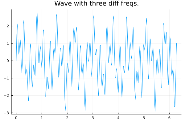
Then plotting the magnitude of the complex DFT vector returned by the fft algorithm we get:
X = fft(y)
plot(abs.(X), label=false, title="DFT same length as y=$(length(y))")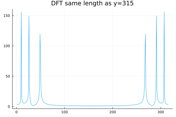
which as you can see indeed multiple peaks but doesn't really line up with the expectation.
For one there are six peaks instead of three for a signal with just three frequencies.
The axis doesn't list any frequencies instead it simply shows the index along the vector.
Regarding the first, we already touch upon the reason. The complex vector returned by fft function for real valued inputs has redundant information because half of it is the complex conjugate of the other half. Therefore when we use the abs function on it, we get twice the number of peaks as there are frequencies.
Regarding the second, let us try to construct the frequency vector and plot it. Now recall that the Nyquist frequency statement: A sampling frequency of at least is needed to capture frequency content up to frequency . Therefore, one expects that for an input of sampling frequency , the DFT will return complex sinusoids with frequencies in properly recovered up to fs/2, therefore for complex vector returned by fft the convention is to make plots with the frequency axis as: [-fs/2, fs/2][1].
Hence, we construct the frequency vector freqs accordingly and normalize by the length of the signal lx while multiplying with the sampling frequency (1/0.02).
lx = length(X)
freqs = (-lx÷2:lx÷2)/lx*50
p1 = plot(freqs, abs.(X), label=false)
vline!(p1, [sqrt(2), 4, sqrt(59)], label="Fundamental freqs.")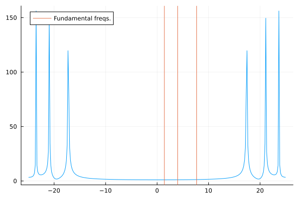
Hmm, is something wrong?
Apart from the obviously missing frequency vector, it also seems the returned DFT matrix orders the components in a certain fashion to speed things up. This infact will be the the case in most FFT implementations.
The way it is sorted is
where is the DC component and is the complex conjugate of .
Fortunately, most implementations also provide a helper function called fftshift which centers the zero frequency for us. Most software packages should provide some implementation of it.
lx = length(X)
freqs = (-lx÷2:lx÷2)/lx*(1/0.02)
p1 = plot(freqs, abs.(fftshift(X)), label=false)
vline!(p1, [sqrt(2), 4, sqrt(59)], label="Fundamental freqs.")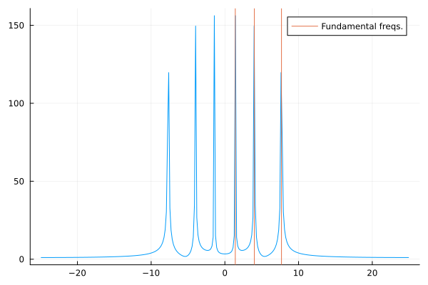
In the next lecture note, we will discuss the effects of sampling and aliasing on the DFT spectrum. In class, we will also get a chance to examine the DFT of a real world signal[2]. In the mean time, here is a pretty cool video from YouTube-r and math popularizer Grant Sanderson[3].
Nice videos on the Fourier Transform
The video below explains the decomposition we have been studying from the perspective of sound waves (pure tones, which are essentially sinusoids). What is a new perspective here though is the small "winding machine" that is introduced to explain the peaks in the frequency-magnitude graphs we have shown so far.
The same channel has a few more videos on the Fourier transform if you are interested. They are a tad bit more involved than the above; particularly because sometimes they are part of a playlist on differential equations or some other advanced topic.
The next video is a very informative video on what is arguably the most important algorithm of our time, the fast Fourier transform.
| [1] | A negative frequency basically corresponds to the complex conjugate of whatever complex exponential was associated to frequency . |
| [3] | Apart from a deep respect for his skill and effort, this course, website or author has no affiliation or relations with Mr. Sanderson or his YouTube channel. |
| [2] | Notebook used available here. |