Lecture 07

Reading material: Section 3.3 - 3.4 (inclusive) of CSSB.

Recap

All of last lecture we spent building up intuition on what Fourier expansions and series do for us. The takeaway was that Fourier series represents a continuous periodic function in terms of a new basis of sines and cosines, and that the Fourier transform was the extension of this to aperiodic signals which allowed us to move between the time domain and frequency domain representations.

In this lecture we will work out a few examples and then present a version of the Fourier transforms that don't involve complex numbers^[1].

Examples

Sine wave

Let us start simple: What is the Fourier series of a simple sine wave: $f(t) = \sin(\omega t)$?

Recall from last lecture that we seek to represent $f(t)$ in terms of complex exponentials.

$$f(t) = \sum \limits _{k=-\infty} ^{\infty} F[k] e^{i k \omega_0 t} \quad \textrm{and} \quad t \in [0, T]$$

Here we can write via Euler's identity that:

so that $F[-1] = \dfrac{1}{2i}$ and $F[1] = \dfrac{-1}{2i}$ and all other Fourier coefficients are zero.

Square wave

Let the square wave of period $T$ and amplitude $1$ be given by:

$$f(t) = \begin{cases} \enskip 1 \qquad & 0 < t \le T/2 \\ -1 \qquad & T/2 < t \le T \end{cases}$$

Then computing its Fourier coefficients we have that:

The indefinite integral evaluates to: which on plugging in the limits evaluates to: Next put $\omega_0 = \dfrac{2 \pi}{T}$ to get: Recall that $k \in \mathbb{Z}$ and note that for every even $k$ the quantity in the parenthesis is zero and so $F[k]=0$ (for $k=0$ need to take a limit). For $k$ that is odd, a small calculation shows that the quantity reduces to $\dfrac{2}{i\pi k}$. Thus,

Triangle wave

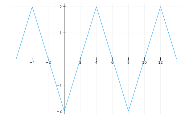
Let us compute the Fourier coefficients of the waveform shown below:

By observation the period of the triangular waveform above is $T=8$ and it traverses its peak-to-peak amplitude of 4 units in 4 seconds. Thus over one period $[0,8]$ we can represent it as:

$$f(t) = \begin{cases} t - 2, \quad & 0< t \le 4 \\ 6 - t, \quad & 4 < t \le 8 \end{cases}$$

Then $\omega_0 = \pi / 4$ and we seek to find the coefficients in the representation

The $F[k]$ are found by: The second and third integrals not requiring integration by parts evaluate to respectively. Note that these are zero for $k$ even. Some coefficients being zero for odd/even $k$ is due to certain symmetries of the function as we will discuss next. The ones that require integration by parts are a bit more involved and quite hairy to do by hand. One can calculate them, using some CAS or MATLAB if necessary (below shown in Mathematica):

In the above, we see that the calculations are only off by a normalizing factor, which will be often the case since different software/systems use differing conventions.

Trigonometric form of Fourier expansions

It is common to write down the Fourier series in terms of the sine and cosine functions separately rather than via the complex exponential^[2]. This is easy to do via Euler's identity. Suppose we can write the Fourier Series expansion for a periodic $f(t)$ as:

$$f(t) = c_0 + \sum \limits_{k=1}^{\infty} a_k \cos(k\omega_0t) + b_k \sin (k\omega_0t)$$

then it is not unreasonable to expect that the above formulation must be related to (1) via Euler's formula. Indeed we can write:

To keep things notation friendly lets represent the $F[-k]$ coefficients as $F_{-k}$. Then we have,

Collect terms one more time to get:

$$F_0 + \sum \limits _{k=1} ^{\infty} \left(F_{-k}+F_{k}\right)\cdot \cos(k \omega_0 t) + i \left(F_{k} - F_{-k}\right) \cdot \sin (k \omega_0 t)$$

Now comparing (5) with (4) we get that:

The above relationship while illuminating, still requires us to compute the complex coefficients first to get to the trigonometric ones. However, we can get the $c_0, a_k$ and $b_k$ directly as:

$$c_0 = \dfrac{2}{T} \int \limits_0 ^T f(t) dt, \quad a_k = \dfrac{2}{T} \int \limits _0 ^T f(t) \cos(k\omega_0 t) dt, \quad b_k = \dfrac{2}{T} \int \limits_0 ^T f(t) \sin(k\omega_0t) dt$$

Common categories of functions

As noted above often some coefficients in the Fourier expansion will turn out to be zero. This can be predicted by looking for specific types of symmetries in a function. Thus we have the following definitions:

Even and odd functions

• A function $f(t)$ is an odd function if $f(-t) = -f(t)$.

• A function $f(t)$ is an even function if $f(-t) = f(t)$.

Based on the above we have that:

1. The sum of two even functions is even, and of two odd ones odd.

2. The product of two even or two odd functions is even.

3. The product of an even and an odd function is odd.

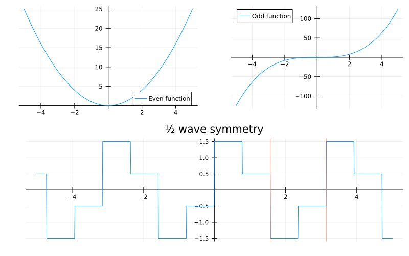
The top plots in the figure below show two classic polynomial examples of odd and even functions.

It is easy to see that symmetries simplify some integrals. For example based on the figures above and considering "area cancellations" or "area additions":

Half and quarter wave symmetries

The definitions for half and quarter wave symmetries apply only to periodic signals.

• A function $f(t)$ periodic with period $T$ is said to exhibit half-wave symmetry if $f(t) = - f(t - T/2)$

• A periodic function $f(t)$ is said to exhibit quarter wave symmetry if in addition to having half-wave symmetry it also has odd/even symmetry.

Thus in the above figure, the bottom plot is an example of a function that exhibits half-wave symmetry.

Question: Does the Mario function in the above figure exhibit quarter-wave symmetry?

Effect of symmetries on Fourier coefficients

Since the sine function is odd and the cosine function is even the integrands in (6) themselves can be odd or even depending on the type of function $f(t)$. These can be understood in terms of area cancellations or additions as alluded to above. Table 3.1 from CSSB summarizes the effect of symmetries on the Fourier sine and cosine coefficients.

Function Type	Symmetry	Coefficient Value
Even	$f(-t) = f(t)$	$b_m=0$
Odd	$f(-t) = -f(t)$	$a_m=0=c_0$
Half-wave	$f(t-T/2)=-f(t)$	$a_m=b_m=0$ for $m$ even

More examples

Square wave (odd)

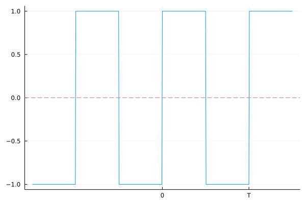
Consider again the square wave from (2). We can verify by plotting the function that it is indeed an odd one.

Thus the coefficients $a_n = c_0 = 0$ and we are left with a Fourier Sine series for this function consisting of only the $b_n$ coefficients. These can be computed as:

It is easy to verify that the final coefficients are zero for $k$ even which dovetails with the fact that the above function also has half-wave symmetry.

Question: Can you derive the $b_k$ coefficients solely based on the complex Fourier series coefficients we calculated in the first set of examples?

Triangle wave (even)

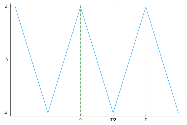
The triangle wave depicted above is even. Thus all the $b_k = 0$. For $c_0$, the average value is also zero by inspection. Thus we are left to compute $a_k$. We have

Now note that in the interval $[0, T/2]$ we can write the function as: $f(t) = \left(A - \dfrac{4At}{T} \right)$. Then, The first integrand on the right is straightforward but the second requires integration by parts. Doing so gives,

It is easy to verify that the above coefficients vanish for even $k$. The first few terms are shown below (compare with earlier derivation using CAS):

Question: (a) Why are the signs different? (b) Why are the even coefficients gone?

While this lecture was mostly analytical, in the next one we will get started with learning more about different software implementations of and related to Fourier Analysis.

[back]

[1]	I hesitate to call it the real transform because neither is more real than the other, except maybe that the complex formulation has several advantages (compactness of notation being the least) over the real one - which we will discuss later.

[2]

Fourier himself passed away in 1830 and it seems it wasn't until 1831 that the great mathematician Gauss delineated the formalism we use today for complex numbers. Therefore it seems likely that for a very long time (and maybe even today) people preferred this second "real" approach that doesn't involve $i$ or $e^i$.