ECE 486 Control Systems
Lecture 23
Joint Observer and Controller Design
Last time we discussed observability and Luenberger observer. Further we talked about state estimation error.
In this lecture, we will go down that line to talk about the joint observer and controller design — dynamic output feedback. We shall learn how to design an observer and a controller to achieve accurate closed-loop pole placement.
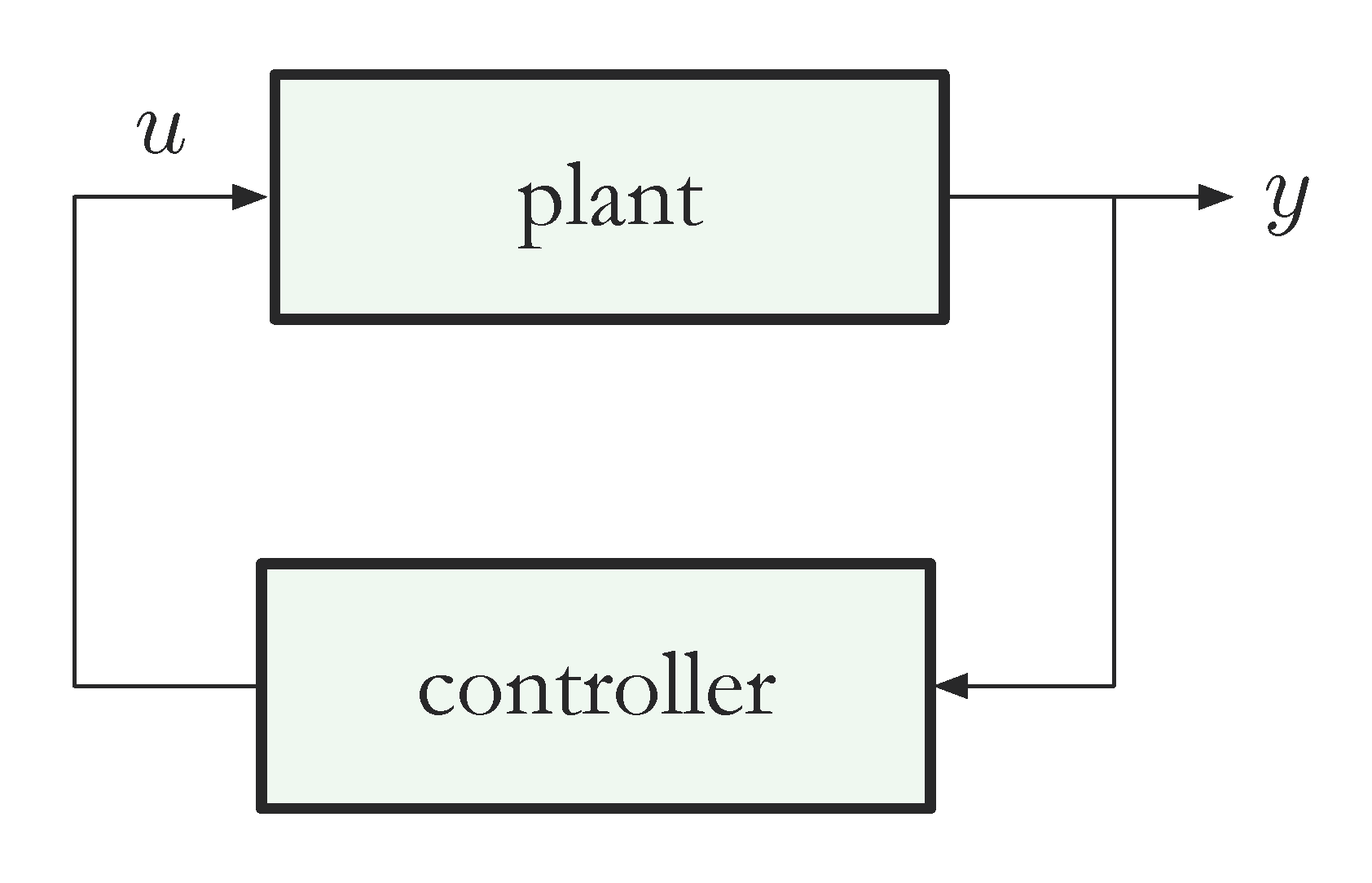
In a typical system, measurements are provided by sensors. In Figure 1, there is not a sensor block between the controller and output \(y\). Therefore, the full state feedback \(u = -Kx\) is not implementable due to the lack of information about internal state \(x\).

Figure 1: Controller only on the feedback path to enclose the open-loop set-up
Recall from last time, an observer is used to estimate the state \(x\). Between output \(y\) and controller, we have an observer block as shown in Figure 2.

Figure 2: The estimate of true state \(x\) using output \(y\) is \(\hat{x}\)
Combining Full-State Feedback with an Observer
So far, we have focused on autonomous systems, i.e., the cases in which input \(u=0\). What about nonzero inputs?
Assuming \((A,B)\) is completely controllable and \((A,C)\) is completely observable, the state-space model
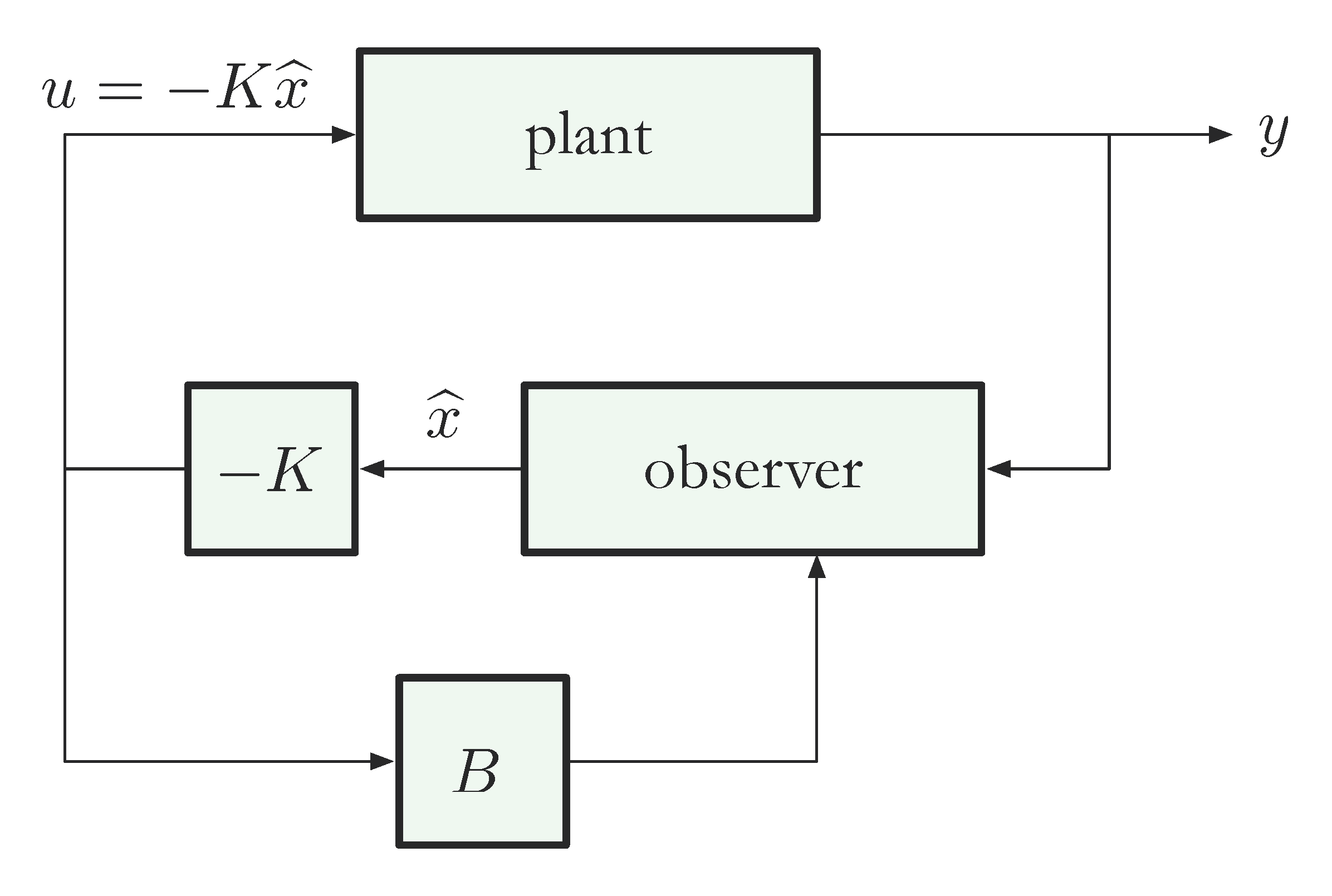
\begin{align*} \dot{x} &= Ax + Bu, \\ y &= Cx \end{align*}in a closed-loop with full state feedback and observer can be implemented as in Figure 3.

Figure 3: Combining state feedback and observer
We know how to find \(K\), such that \(A-BK\) has desired eigenvalues, i.e., pole placement for the controller. The difficulty here is since we do not have access to \(x\), we must design an observer. And this time, we need a slight modification because of the not necessarily zero \(Bu\) term.
Observer in the Presence of Control Input
First let’s see what goes wrong when we use the old approach
\begin{align*} \dot{\widehat{x}} &= (A-LC)\widehat{x} + Ly. \end{align*}For the estimation error \(e = x - \widehat{x}\), we have
\begin{align*} \dot{e} &= \dot{x} - \dot{\widehat{x}} \\ &= Ax + Bu - \left[(A-LC)\widehat{x} + LCx\right] \\ &= (A-LC)e + Bu. \tag{1} \label{d23_eq1} \end{align*}If \(u \neq 0\), then \(Bu\) is not necessarily \(0\) either. Then \(e(\infty) = 0\) is no longer necessarily a steady state solution to Equation \eqref{d23_eq1}, meaning, even if \(e(t)\) converges as \(t \to \infty\), it may not converge to zero. There might be a constant estimation error.
However, it is easy to correct this. Since \(u\) is a signal we can access, let’s use it as an input to the observer to cancel the \(Bu\) term from \(\dot{x}\).
If we try the modified observer structure,
\begin{align*} \dot{\widehat{x}} &= (A-LC)\widehat{x} + Ly + Bu \\ \dot{e} &= \dot{x} - \dot{\widehat{x}} \\ &= Ax + Bu - \left[(A-LC)\widehat{x} + LCx + Bu\right] \\ &= (A-LC)e. \end{align*}We see that \(Bu\) term is gone in the dynamics of \(e\). Then we have three dynamics equations regarding the plant, the observer and the estimation error respectively.
\begin{align*} \text{System: } \, & \dot{x} = Ax + Bu, \\ & y = Cx. \\ \text{Observer: } \, & \dot{\widehat{x}} = (A-LC)\widehat{x} + Ly + Bu. \\ \text{Error: } \, & \dot{e} = (A-LC)e. \end{align*}By observability, we can arbitrarily assign the eigenvalues of \(A-LC\). These eigenvalues should be farther into LHP since we want the error to decay to zero fast.
By controllablity, we can arbitrarily assign the eigenvalues of \(A-BK\).
The resulting controller based on estimated state \(\hat{x}\) is therefore
\begin{align*} u = - K\widehat{x} \quad \text{(estimated state feedback)} \end{align*}and the overall observer-controller system is
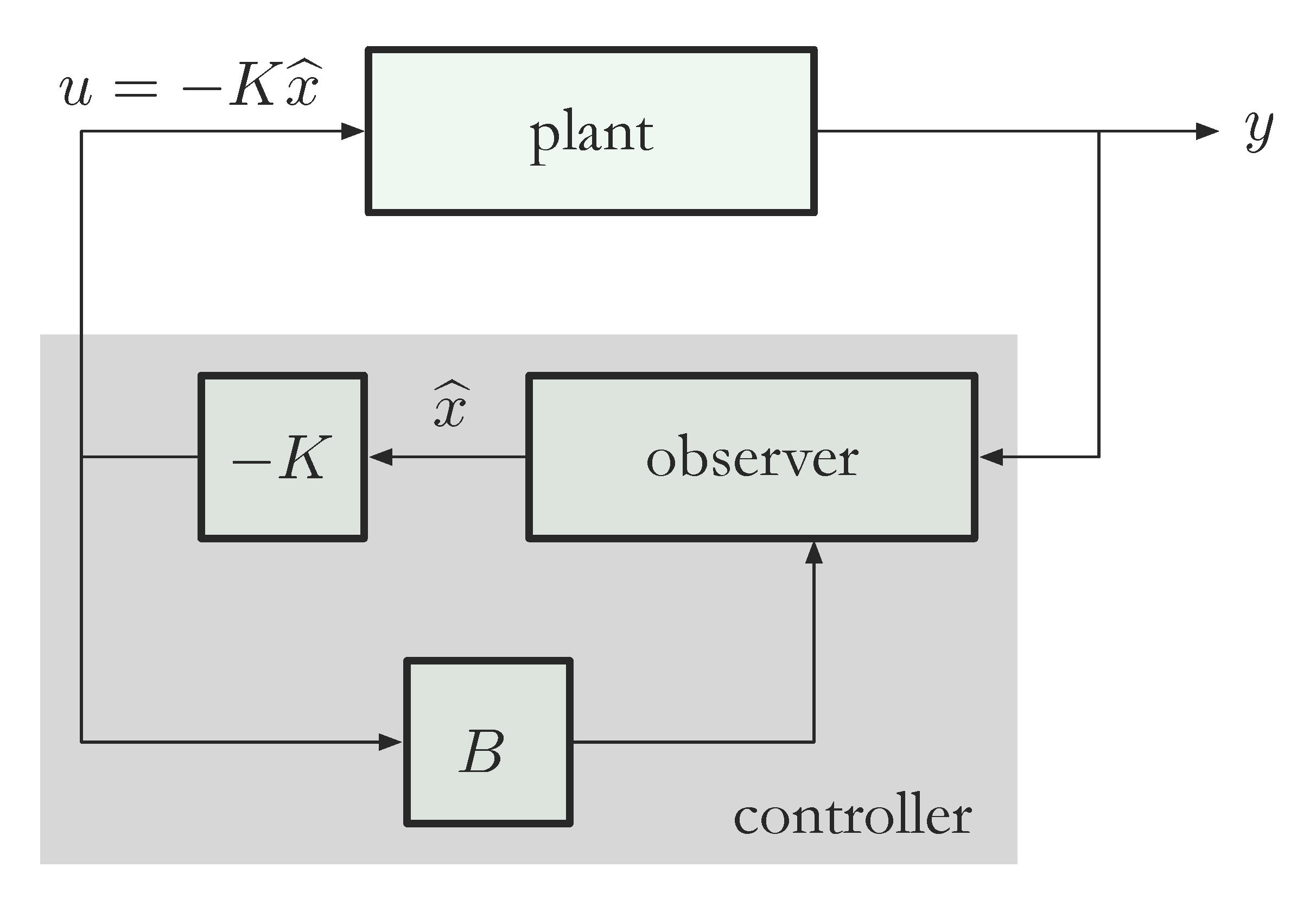
\begin{align*} \dot{\widehat{x}} &= (A-LC)\widehat{x} + Ly + B\underbrace{(-K\widehat{x})}_{=u} \\ &= (A-LC - BK)\widehat{x} + Ly, \\ u &= - K\widehat{x}. \hspace{5cm} \text{(dynamic output feedback)} \end{align*}We notice that this is a dynamical system with input \(y\) (the output of state-space model) and output \(u\) (the input to state-space model).
The observer-controller subsystem is highlighted in Figure 4.

Figure 4: Dynamic output feedback
To compute the transfer function from \(y\) to \(u\), we follow the calculation as follows. Apply Laplace transform to observer-controller subsystem
\begin{align*} \dot{\widehat{x}} &= (A-LC-BK)\widehat{x} + Ly, \\ u &= -K\widehat{x} \end{align*}we get
\begin{align*} s\widehat{X} &= (A-LC-BK)\widehat{X} + LY, \\ U &= -K\widehat{X}. \\ \implies U &= \underbrace{-K(sI-A+LC+BK)^{-1}L}_{:=D(s)}Y. \end{align*}The transfer function is therefore \(D(s) = -K(sI-A+LC+BK)^{-1}L\).
Dynamic Output Feedback: Does It Work?
When \(y=x\), i.e., the true state \(x\) can be obtained via measurements \(y\), the full state feedback control input \(u=-Kx\) achieves desired pole placement.
How do we know that using control based on estimates, \(u=-K\widehat{x}\) achieves similar objectives?
Here is our overall closed-loop system,
\begin{align*} \dot{x} &= Ax - BK\widehat{x}, \\ \dot{\widehat{x}} &= (A-LC-BK)\widehat{x} + LCx. \end{align*}We can write it in block matrix form to augment the system state-space model
\begin{align*} \tag{2} \label{d23_eq2} \left( \begin{matrix} \dot{x} \\ \dot{\widehat{x}} \end{matrix}\right) = \left( \begin{matrix} A & -BK \\ LC & A-LC-BK \end{matrix}\right)\left( \begin{matrix} x \\ \widehat{x} \end{matrix}\right). \end{align*}How do we relate this to the “nominal” closed-loop behavior, i.e., what is the relationship between the augmented block matrix in Equation \eqref{d23_eq2} and \(A-BK\)?
If we use linear transformation to convert \(\left( \begin{array}{c} x \\ \widehat{x} \end{array}\right)\) to \(\left( \begin{array}{c} x \\ e \end{array}\right)\), we get
\begin{align*} \left( \begin{matrix} x \\ \widehat{x} \end{matrix}\right) \mapsto \left( \begin{matrix} x \\ e \end{matrix}\right) &= \left( \begin{matrix} x \\ x-\widehat{x} \end{matrix}\right) \\ &= \underbrace{\left( \begin{matrix} I & 0 \\ I & -I \end{matrix}\right)}_{T} \left( \begin{matrix} x \\ \widehat{x} \end{matrix}\right). \end{align*}We notice
- The transformation matrix \(T\) is invertible (Why? Hint: \(T\) is lower triangular, \(\det (T)\) is the product of diagonal entries), so the new representation is equivalent to the old one.
In the new coordinates, we have
\begin{align*} \dot{x} &= Ax - BK\widehat{x} \\ &= (A-BK)x + BK(x-\widehat{x}) \\ \tag{3} \label{d23_eq3} &= (A-BK)x + BK e, \\ \dot{e} &= (A-LC)e. \tag{4} \label{d23_eq4} \end{align*}
Equations \eqref{d23_eq3} and \eqref{d23_eq4} give us the representation by the so called separation principle.
So now we can write
\begin{align*} \left( \begin{matrix} \dot{x} \\ \dot{e} \end{matrix}\right) &= \underbrace{\left( \begin{matrix} A - BK \, & \, BK \\ 0 \, & \, A-LC \end{matrix}\right)}_{\text{upper triangular matrix}} \left( \begin{matrix} x \\ e \end{matrix}\right). \end{align*}The closed-loop characteristic polynomial is
\begin{align*} \tag{5} \label{d23_eq5} \det \left( \begin{matrix} sI - A + BK \, & \, -BK \\ 0 \, & \, sI - A+LC \end{matrix}\right) = \det \left(sI-A+BK\right) \cdot \det\left(sI-A+LC\right). \end{align*}By Equation \eqref{d23_eq5}, separation principle says the closed-loop eigenvalues are
\begin{align*} &\Big\{ \text{controller poles, i.e., roots of $\det(sI-A+BK)$} \Big\} \\ &\,\,\bigcup \Big\{ \text{observer poles, i.e., roots of $\det(sI-A+LC)$} \Big\}. \end{align*}Bear in mind this holds only for linear systems.
Summary: The moral of the story
- If we choose observer poles to be several times faster than the controller poles, e.g., 2 – 5 times further away origin, then the controller poles will be dominant.
- Dynamic output feedback gives essentially the same performance as (nonimplementable) full-state feedback — provided the observer poles are far enough into LHP so the estimation error decays fast enough to \(0\).
- The necessary condition though is the system must be completely controllable and completely observable.