ECE 486 Control Systems
Lecture 22

[486 Home]
Prev	ECE 486 Handbook	Next

State Estimation and Observer

Last time, we saw the technique of arbitrary pole placement by full state feedback. Today, we will learn observer design for state estimation when full state feedback is not implementable.

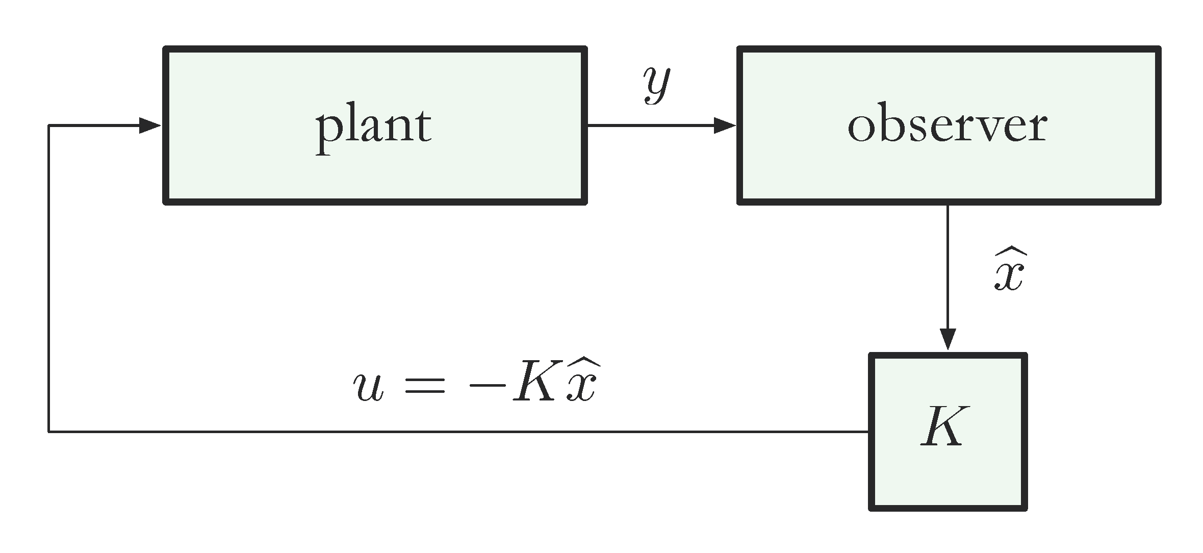
For observable systems (see definition below), we estimate the state $x$ from output $y=Cx$ using an observer. In case the true state is not available for us to build controller $u = -Kx$, with its estimate $\hat{x}$ at our disposal, we can use $\hat{x}$ instead. Then the controller takes the form $u = -K\hat{x}$.

State Estimation Using an Observer

When full state feedback is unavailable, an observer is used to estimate the state $x$.

estimate xhat

Figure 1: The estimate of true state $x$ using output $y$ is $\hat{x}$

The idea is to design the observer in such a way that the state estimate $\widehat{x}$ is asymptotically accurate.

\begin{align*} \| \widehat{x}(t) - x(t) \| &= \sqrt{\sum^n_{i=1} \big(\widehat{x}_i(t) - x_i(t)\big)^2} \\ & \to 0, \, \text{ as } t \to \infty. \end{align*}

If we are successful, then we can try estimated state feedback:

control via xhat

Figure 2: Controller based on the estimate of true state $x$ using output $y$

Observability Matrix

Last time, we saw that closed-loop poles can be assigned arbitrarily by full state feedback when the plant is completely controllable.

Now, we shall see that asymptotically accurate state estimation will be possible when the system is completely observable.

Observability in fact is a system property which is dual to controllability.

Consider a single-output system with $y \in \RR^1$.

\begin{align*} \dot{x} &= Ax + Bu, \\ y &= Cx, \end{align*}

where $x \in \RR^n$. The Observability Matrix is defined as

\begin{align*} \tag{1} \label{d22_eq1} {\cal O}(A,C) = \left[ \begin{matrix} C \\ CA \\ \vdots \\ CA^{n-1} \end{matrix} \right]. \end{align*}

Recall that $C$ is $1 \times n$ and $A$ is $n \times n$, so ${\cal O}(A,C)$ is $n \times n$. The observability matrix only involves $A$ and $C$, not $B$.

We say that the above system is completely observable if its observability matrix ${\cal O}(A,C)$ is invertible.

This definition is only true for the single-output case. It can be generalized to the multiple-input case using the rank of observability matrix ${\cal O}(A,C)$.

Example: Computing the observability matrix ${\cal O}(A,C)$ given

\begin{align*} A = \left( \begin{matrix} 0 & - 6 \\ 1 & -5 \end{matrix}\right), \, C = \left( \begin{matrix} 0 & 1 \end{matrix}\right). \end{align*}

Solution: Here, the given matrices are for a single output system with two states, i.e., $n=2$, $C \in \RR^{1 \times 2}, A \in \RR^{2\times 2}$. Therefore ${\cal O}(A,C) \in \RR^{2 \times 2}$.

By the definition of observability matrix in Equation \eqref{d22_eq1},

\begin{align*} {\cal O}(A,C) = \left[ \begin{matrix} C \\ CA \end{matrix}\right], \end{align*}

where

\begin{align*} CA &= \left( \begin{matrix} 0 & 1 \end{matrix}\right) \left( \begin{matrix} 0 & - 6 \\ 1 & -5 \end{matrix}\right) \\ &= \left( \begin{matrix} 1 & -5 \end{matrix}\right). \\ \implies {\cal O}(A,C) &= \left( \begin{matrix} 0 & 1 \\ 1 & -5 \end{matrix}\right). \end{align*}

We notice $\det {\cal O}(A,C) = - 1 \neq 0$, hence the system is completely observable.

The given matrices $A,C$ of the system are in Observable Canonical Form (OCF).

Observable Canonical Form

A single-output state-space model

\begin{align*} \dot{x} &= Ax + Bu, \\ y &= Cx \end{align*}

is said to be in Observable Canonical Form (OCF) if the matrices $A,C$ are of the form

\begin{align*} A &= \left( \begin{matrix} 0 & 0 & \ldots & 0 & 0 & * \\ 1 & 0 & \ldots & 0 & 0 & * \\ \vdots & \vdots & \ddots & \vdots & \vdots & \vdots \\ 0 & 0 & \ldots & 1 & 0 & * \\ 0 & 0 & \ldots & 0 & 1 & * \end{matrix} \right), \\ C &= \left( \begin{matrix} 0 & 0 & \ldots & 0 & 1 \end{matrix}\right). \end{align*}

Note that a system in OCF is always observable.

The proof of this for $n > 2$ uses the Jordan canonical form, we shall not worry about this. Interested readers can follow the underlined link.

Coordinate Transformations and Observability

Similar to controllability, observability is preserved under invertible coordinate transformations.

Under the linear transform $\tau : x \mapsto Tx$, we have

\begin{align*} \begin{array}{l} \dot{x} = Ax + Bu,\\ y = Cx, \end{array} \quad \xrightarrow{\quad T \quad} \quad \begin{array}{l} \dot{\bar{x}} = \bar{A}\bar{x} + \bar{B}u, \\ y = \bar{C}\bar{x}, \end{array} \end{align*}

where

\begin{align*} \bar{A} = TAT^{-1}, \, \bar{B} = TB, \, \bar{C} = CT^{-1}. \end{align*}

Claim: Observability does not change under linear transformation.

Proof: For any $k = 0,1,\ldots$, note by induction

\begin{align*} \bar{C}\bar{A}^k &= CT^{-1}(TAT^{-1})^k \\ &= CT^{-1} TA^{k}T^{-1} \\ &= CA^kT^{-1}. \end{align*}

Therefore,

\begin{align*} {\cal O}(\bar{A},\bar{C}) &= \left( \begin{matrix} \bar{C} \\ \bar{C}\bar{A} \\ \vdots \\ \bar{C}\bar{A}^{n-1} \end{matrix}\right) \\ &= \left( \begin{matrix} CT^{-1} \\ CT^{-1}TAT^{-1} \\ \vdots \\ CT^{-1}TA^{n-1}T^{-1} \end{matrix}\right) \\ &= \left( \begin{matrix} C \\ CA \\ \vdots \\ CA^{n-1} \end{matrix}\right)T^{-1} \\ &= {\cal O}(A,C) T^{-1}. \end{align*}

Since $\det T \neq 0$, $\det {\cal O}(\bar{A},\bar{C}) \neq 0$ if and only if $\det {\cal O}(A,C) \neq 0$.

Thus, the new system is completely observable if and only if the original one is.

If the original system is observable, then from the above proof of the invariance of observability, we obtain a formula for the linear transform $T$.

\begin{align*} & T\underbrace{\left[ {\cal O}(A,C)\right]^{-1}}_{\text{old}} = \underbrace{\left[{\cal O}(\bar{A},\bar{C})\right]^{-1}}_{\text{new}} \\ \implies & T = \underbrace{\left[{\cal O}(\bar{A},\bar{C})\right]^{-1}}_{\text{new}}\underbrace{\left[ {\cal O}(A,C)\right]}_{\text{old}}. \end{align*}

As we will show next,

Theorem: If the system is observable, then there exists an observer (state estimator) that provides an asymptotically convergent estimate $\widehat{x}$ of the state $x$ based on the observed output $y$.

control via xhat

Figure 3: David Luenberger

Remark: This particular type of observer we will construct is also called the Luenberger observer after David G. Luenberger, who developed this idea in his 1963 Ph.D. dissertation. David Luenberger is a Professor at Stanford University.

Luenberger Observer

Consider a state-space model, (assuming for now, $u=0$)

\begin{align*} \dot{x} &= Ax, \\ y &= Cx. \end{align*}

We wish to estimate the state $x$ based on the output $y$.

Consider feeding the output $y$ as input to the following system with state $\widehat{x}$:

\begin{align*} \tag{2} \label{d22_eq2} \dot{\widehat{x}} = (A-LC)\widehat{x} + L y. \end{align*}

Note the output injection matrix $L$ in Equation \eqref{d22_eq2} is chosen such that the matrix $A-LC$ is Hurwitz, i.e., all of its eigenvalues lie in Left Half Plane.

At this point, we do not assume anything about observability.

Then on top of the system state-space model, we have one more dynamics equation for the observer.

\begin{align*} \text{System: } \,& \dot{x} = Ax, \\ &y = Cx. \\ \text{Observer: } \, & \dot{\widehat{x}} = (A-LC)\widehat{x} + L y. \end{align*}

Estimation Error

We are interested in the state estimation error $e = x - \widehat{x}$ as $t \to \infty$, since it tells us how accurate our estimate is over time. The error dynamics is governed by the differential equation

\begin{align*} \dot{e} &= \dot{x} - \dot{\widehat{x}} \\ &= Ax - \left[(A-LC)\widehat{x} + LCx \right] \\ &= (A-LC) x - (A-LC)\widehat{x} \\ &= (A-LC)e. \end{align*}

We wish to see $e(t)$ converge to zero in some sense.

Linear ODEs and Eigenvalues: Let’s briefly recall, consider a system dynamics equation

\begin{align*} \dot{v} &= Fv, \text{ where } v \in \RR^n, F \in \RR^{n \times n}. \end{align*}

Let $\lambda_1,\ldots,\lambda_n$ be the eigenvalues of matrix $F$, i.e., roots of $\det(sI-F) = 0$.

If matrix $F$ is diagonalizable, then there exists a matrix $T \in \RR^{n \times n}$, such that $T^{-1}=T^T$ ($T$ is orthogonal in this case) and

\[ F = T^{-1} \left( \begin{matrix} \lambda_1 & \\ & \lambda_2 \\ && \ddots \\ &&& \lambda_n \end{matrix}\right) T. \]

Use the change of coordinates $\bar{v} = Tv$. Then

\begin{align*} \tag{3} \label{d22_eq3} \dot{\bar{v}} &= TFT^{-1}\bar{v} = \left( \begin{matrix} \lambda_1 & \\ & \lambda_2 \\ && \ddots \\ &&& \lambda_n \end{matrix}\right)\bar{v}. \end{align*}

Write down the equations row-wise in Equation \eqref{d22_eq3}, we have

\begin{align*} \dot{\bar{v}}_i &= \lambda_i \bar{v}_i, \forall~ i = 1,2,\ldots,n. \end{align*}

For each $i$, $1 \leq i \leq n$, the first order ODE has the solution

\begin{align*} \bar{v}_i(t) &= \bar{v}_i(0) e^{\lambda_i t}. \end{align*}

If in addition, all $\lambda_i$’s have negative real parts, then

\begin{align*} \| v(t) \|^2 &= v(t)^Tv(t) \\ &= \bar{v}(t)^T\bar{v}(t) \\ &\le Ce^{-2\sigma_{\min}t}, \end{align*}

where $\sigma_{\min} = \min_{1 \le i \le n} |{\rm Re}(\lambda_i)|$. It says the norm of $v(t)$ is bounded by an exponential associated with the slowest decaying mode times some constant depending on $n$.

Recall our assumption that the matrix $A-LC$ is Hurwitz, i.e., all its eigenvalues are in LHP, ${\rm Re} (\lambda_i) <0$ for all eigenvalues of $A-LC$. By the above note on solutions to a system of ODEs, this implies that estimation error

\begin{align*} \|x(t) - \widehat{x}(t) \|^2 &= \| e(t) \|^2 \\ &= \sum^n_{i=1} |e_i(t)|^2\\ & \to 0, \text{ as } t \to \infty. \end{align*}

at an exponential rate, determined by the eigenvalues of $A-LC$.

Therefore, for fast convergence of estimation error to zero (meaning estimation $\hat{x}$ converging to true state $x$), we want the eigenvalues of $A-LC$ to be far into the Left Half Plane.

We further notice by Equation \eqref{d22_eq2}, the input-output relationship from $Y(s)$ to $\hat{X}(s)$ (using measurements to obtain estimates) can be derived as

\begin{align*} s\hat{X}(s) &= (A-LC)\hat{X}(s) + LY(s) \\ \implies LY(s) &= (sI-A+LC)\hat{X}(s) \\ \hat{X}(s) &= (sI-A+LC)^{-1}L Y(s). \end{align*}

The eigenvalues of $A-LC$ are the observer poles. We want these poles to be stable and fast in the sense of making estimation error go to zero.

Observability and Observer Pole Placement

If the system

\begin{align*} \dot{x} &= Ax, \\ y &= Cx \end{align*}

is completely observable, then we can arbitrarily assign the eigenvalues of $A-LC$ by a suitable choice of the output injection matrix $L$.

In comparison, this is similar to the fact that controllability implies arbitrary closed-loop pole placement by state feedback $u = -Kx$.

In fact, these two facts are closely related because CCF is dual to OCF.

Indeed, consider a single-output system in OCF with $y \in \RR^1$,

\begin{align*} \dot{x} &= Ax \\ y &= Cx, \\ \text{where } A &= \left( \begin{matrix} 0 & 0 & \ldots & 0 & 0 & -a_n \\ 1 & 0 & \ldots & 0 & 0 & -a_{n-1} \\ \vdots & \vdots & \ddots & \vdots & \vdots & \vdots \\ 0 & 0 & \ldots & 1 & 0 & -a_{2} \\ 0 & 0 & \ldots & 0 & 1 & -a_1 \end{matrix} \right), \\ C &= \left( \begin{matrix} 0 & 0 & \ldots & 0 & 1 \end{matrix}\right). \end{align*}

Note that $A^T$ is in the form of a CCF system. Then

\begin{align*} \det(sI-A) &= \det((sI-A)^T) \hspace{3cm} \text{(by $\det(M) = \det(M^T)$)}\\ &= \det(sI-A^T) \hspace{3.5cm}\text{(by $(M_1+M_2)^T = M_1^T + M_2^T$)}\\ \tag{4} \label{d22_eq4} &= s^n + a_1 s^{n-1} + \cdots + a_{n-1}s + a_n. \end{align*}

With added output injection matrix $L$, $A - LC$ is still in the same form as $A$. Indeed, the elements of $L$ only enter the last column of $A$ one at a time (cf. entries of $K$ enter the last row when we considered the CCF with pole placement.)

\begin{align*} A&= \left( \begin{matrix} 0 & \ldots & 0 & -a_n \\ 1 & \ldots & 0 & -a_{n-1} \\ \vdots & \ddots & \vdots & \vdots \\ 0 & \ldots & 1 & -{a_1} \end{matrix} \right), \\ LC &= \left( \begin{matrix} \ell_1 \\ \ell_2 \\ \vdots \\ \ell_n \\ \end{matrix}\right) \left(\begin{matrix} 0 & 0 & \ldots & 1 \end{matrix}\right) \\ &= \left( \begin{matrix} 0 & \ldots & 0 & \ell_1 \\ 0 & \ldots & 0 & \ell_2 \\ \vdots & \ddots & \vdots & \vdots \\ 0 & \ldots & 0 & \ell_n \end{matrix} \right), \\ A - LC &= \left( \begin{matrix} 0 & \ldots & 0 & -(a_n+\ell_1) \\ 1 & \ldots & 0 & -(a_{n-1}+\ell_2) \\ \vdots & \ddots & \vdots & \vdots \\ 0 & \ldots & 1 & -(a_1 + \ell_n) \end{matrix} \right). \end{align*}

We observe the eigenvalues of $A-LC$ are the roots of the characteristic polynomial by Equation \eqref{d22_eq4}

\begin{align*} &\det(sI-A+LC) \\ &= s^n + (a_1+\ell_n)s^{n-1} + \cdots + (a_{n-1}+\ell_2)s + (a_n+\ell_1). \end{align*}

Observation: When the system is in Observable Canonical Form (OCF), each entry of output injection matrix $L$ affects one and only one of the coefficients of the characteristic polynomial, which can be assigned arbitrarily by a suitable choice of $\ell_1,\ldots,\ell_n$.

Hence the name Observer Canonical Form — convenient for observer design.

We can summarize the general procedure for any completely observable system.

Convert state-space model of the system to OCF using a suitable invertible coordinate transformation given by $T = \underbrace{{\cal O}(\bar{A},\bar{C})^{-1}}_{\text{new}}\underbrace{\left[ {\cal O}(A,C)\right]}_{\text{old}}$.
Find an $\bar{L}$ such that $\bar{A} - \bar{L}\bar{C}$ has desired eigenvalues for the observer.
Convert the solution back to original coordinates then $L = T^{-1}\bar{L}$.

Then the resulting observer is

\begin{align*} \dot{\widehat{x}} = (A-T^{-1}\bar{L}C)\widehat{x} + T^{-1}\bar{L}y. \end{align*}

But this procedure is not absolutely necessary because of duality between controllability and observability.

Claim: (Controllability–Observability Duality) The system

\begin{align*} \dot{x}&= Ax, \\ y &= Cx \end{align*}

is completely observable if and only if the system

\begin{align*} \tag{5} \label{d22_eq5} \dot{x} &= A^Tx + C^Tu \end{align*}

is completely controllable.

Proof: The controllability matrix of system in Equation \eqref{d22_eq5} is computed as

\begin{align*} {\cal C}(A^T,C^T) &= \left[ C^T\, |\, A^T C^T\, |\, \cdots \,|\, (A^T)^{n-1}C^T\right] \\ &= \left[ \begin{matrix} C \\ CA \\ \vdots \\ CA^{n-1} \end{matrix} \right]^T \\ &= \left[{\cal O}(A,C)\right]^T. \end{align*}

Thus ${\cal O}(A,C)$ is nonsingular if and only if ${\cal C}(A^T,C^T)$ is.

Using the controllability-observability duality, the procedure of observer pole placement can be also summarized as: Given a completely observable pair $(A,C)$,

For $F = A^T$, $G = C^T$, consider the system

\[\dot{x} = Fx + Gu.\]

Note this system is completely controllable by duality.
Use the procedure for completely controllable systems to find a $K$ so that

\[ F - GK = A^T - C^TK \]

has desired eigenvalues.
Then
\begin{align*} {\rm eig}(A^T-C^TK) &= {\rm eig}(A^T - C^TK)^T \\ &= {\rm eig}(A-K^TC), \end{align*}
so $L = K^T$ is the desired output injection matrix.

Therefore, the resulting observer is

\begin{align*} \dot{\widehat{x}} &= (A-LC)\widehat{x} + Ly \\ &= (A-\underbrace{K^T}_L C)\widehat{x} + \underbrace{K^T}_L y. \end{align*}

Note that the above observer specified in Equation \eqref{d22_eq2} was based on zero input $u$ in a state-space model.

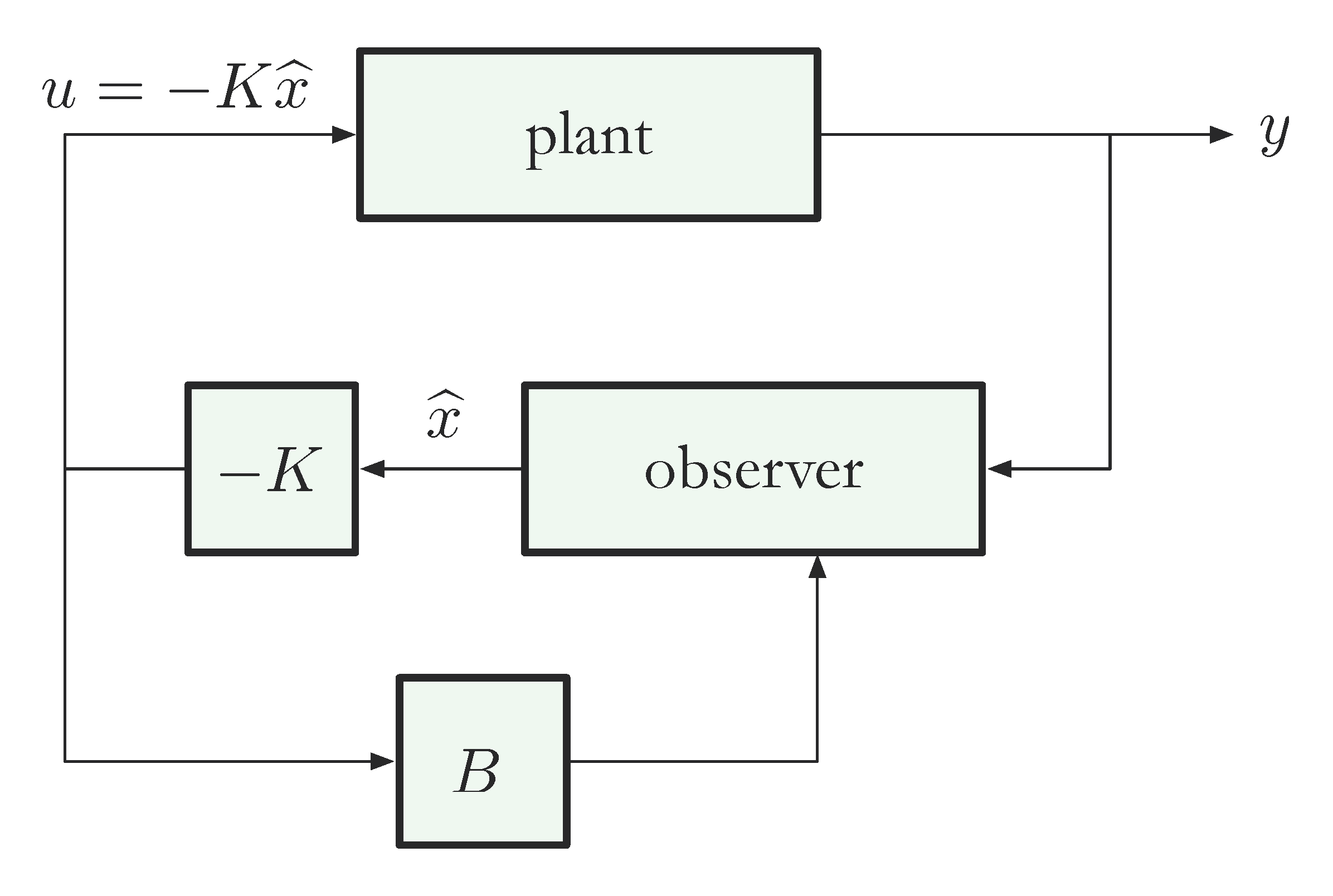
We shall see in the next lecture that assuming $(A,B)$ is completely controllable and $(A,C)$ is completely observable, for the state-space model with not necessarily zero input $u$,