ECE 486 Control Systems
Lecture 11
Root Locus Method (Continued)
We shall continue our discussion of sketching root locus in this lecture. Recall from last time, we introduced the concept of root locus and four (Rules A — D) of the six rules for sketching root locus of \(1 + KL(s)\) given \(L(s) = \frac{b(s)}{a(s)}\), where \(L(s)\) is a proper rational function.
Further we will see how to use Root Locus Design for dynamic compensation, how to use Root Locus in control system stabilization, time response shaping and how to visualize the effect of various controller types on system performance.
Recall the root locus of \(1 + KL(s)\), where
\[L(s) = \dfrac{b(s)}{a(s)} = \dfrac{s^m + b_1 s^{m-1} + \cdots + b_{m-1}s + b_m}{s^n + a_1 s^{n-1} + \cdots + a_{n-1}s + a_n},\, m \le n, \]

Figure 1: Block diagram for Evans Root Locus method
is the set of all \(s \in \CC\) that solve the characteristic equation \[ a(s) + Kb(s) = 0 \] as \(K\) varies from \(0\) to \(\infty\).
Or equivalently by phase condition, the root locus of \(1 + KL(s)\) is the set of all \(s \in \CC\), such that \(\angle L(s) = \pm 180^\circ\), i.e., \(L(s)\) is real and negative.
Rules for Sketching Root Loci (Rules E — F)
Recall the six rules for sketching the root locus,
- Rule A — number of branches (= number of open loop poles)
- Rule B — start points (= open loop poles)
- Rule C — end points (= open loop zeros)
- Rule D — real locus (located relative to real open-loop poles/zeros)
- Rule E — asymptotes
- Rule F — $jω$-crossings
We covered Rules A – D last time.
Rule E: Asymptotes
When \(s \to \infty\), how does the locus look like at infinity? By phase condition,
\begin{align*} 180^\circ &= \angle L(s) \\ &= \angle \frac{s^m + b_1 s^{m-1} + \cdots}{s^n + a_1 s^{n-1} + \cdots} \\ &= \angle\frac{\color{red}{s^{m-n}} + b_1 s^{m-n-1} + \cdots}{1 + a_1 s^{-1} + \cdots} \\ & \to \angle s^{m-n}, \,\,\, \text{if } |s| \to \infty. \hspace{3cm} \text{(by $m\le n$)} \end{align*}Claim: If \(\angle s^{m-n} = 180^\circ\), then \[ \angle s = \frac{180^\circ + \ell \cdot 360^\circ}{n-m}, \qquad \ell = 0,1,\ldots,n-m-1. \]
Proof: Recall for an \(s \in \CC\), its polar form is
\[ s = |s| e^{j \angle s}. \] Then raise \(s\) to $(m-n)$-th power, we have
\begin{align*} s^{m-n} &= |s|^{m-n}e^{j(m-n)\angle s}, \\ (m-n)\angle s &= 180^\circ \implies (m-n)\angle s = 180^\circ + \ell \cdot 360^\circ. \end{align*}Divide out \(m - n\) on both sides then we complete the proof.
Rule E: Branches of root locus at \(\infty\) have phase
\begin{align*} \angle s &\approx \frac{180^\circ + \ell \cdot 360^\circ}{n-m} \\ &= \frac{(2\ell + 1) \cdot 180^\circ}{n-m}, \qquad \ell = 0,1,\ldots,n-m-1. \end{align*}Note: If \(m=n\), then there are no branches at \(\infty\). All \(n\) branches start at open loop poles and end at open loop zeros.
Rule F: $jω$-crossings
Do the branches of the root locus cross the imaginary axis $jω$-axis, i.e., closed loop poles transitioned from Left Half Plane (stability) to Right Half Plane (instability)?
When this transition happens, closed loop poles lie on the imaginary axis, \(s = j\omega\) must satisfy the characteristic equation,
\[ \tag{1} \label{d11_eq1} a(j\omega) + Kb(j\omega) = 0. \]
Therefore it shall have a solution \(\omega \ge 0\) for some \(K > 0\).
Trick: To figure out such $jω$-crossings, we can use the Routh test to first determine the critical value of \(K\) when the characteristic polynomial is about to become unstable. Then plug this \(K\) back into Equation \eqref{d11_eq1} and solve for $jω$-crossings.
We shall complete the unfinished Example 2 in Lecture 10 after we apply Rules E and F.
Example 2 (Lecture 10, continued): Consider the root locus with \[L(s) = \dfrac{s+1}{s(s+2)\big((s+1)^2+1\big)}.\]
Use Rules A — F to sketch its root locus.
Solution: The equivalent open loop transfer function \(L(s)\) is given and we note
- By Rule A, the degree of its denominator is \(4\), hence the root locus has four branches.
- By Rule B, its branches start at open-loop poles \(s = 0\), \(s=-2\), and \(s=-1 \pm j\).
By Rule C, one of its branches ends at open-loop zeros \(s = -1\); three other branches end at \(\pm\infty\) because the degree of its numerator is \(1\).
As a start, we can mark down the poles and zeros that are on the root locus at the moment.
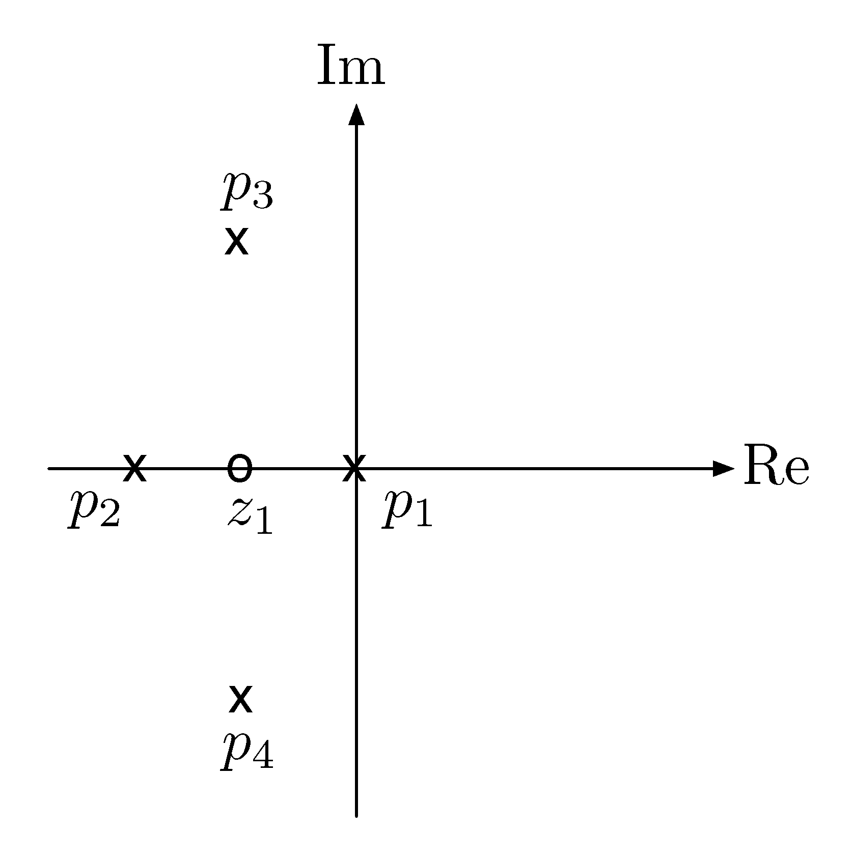
Figure 2: Root locus of $L(s) = \frac{s+1}{s(s+2)\big( (s+1)^2+1 \big)} $, by Rules B and C.
By Rule D, the root locus on the real axis has odd number of real open loop poles and zeros to its right.
Hence we have the root locus on the real axis highlighted in blue.
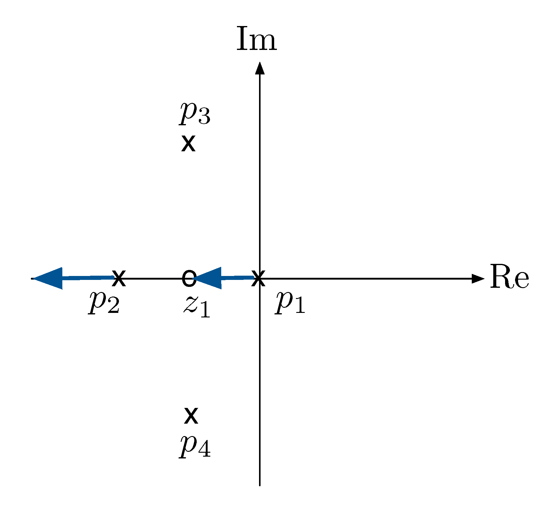
Figure 3: Root locus, Rule D
By Rule E, as for the asymptotes, near \(\infty\) branches of root locus have phase
\begin{align*} \angle s = \frac{(2\ell + 1) \cdot 180^\circ}{n-m}, \qquad \ell = 0,1,\ldots,n-m-1. \end{align*}In this example, \(n=4\) and \(m=1\) for
\[\dfrac{s+1}{s(s+2)\big((s+1)^2+1\big)}.\]
Let \(\ell = 0, 1, 2\). Compute \(\angle s = \frac{(2\ell + 1) \cdot 180^\circ}{3}\).
\begin{align*} \ell = 0: \qquad & \frac{2 \cdot 0 + 1}{3}180^\circ = 60^\circ, \\ \ell = 1: \qquad & \frac{2 \cdot 1 + 1}{3}180^\circ = 180^\circ, \\ \ell = 2: \qquad & \frac{2 \cdot 2 + 1}{3}180^\circ = \frac{5}{3} 180^\circ = \left( 2 - \frac{1}{3} \right)180^\circ = -60^\circ. \end{align*}There are three asymptotes which have angles \(60^\circ,\, 180^\circ,\, -60^\circ\) respectively.
By Rule F, compute the $jω$-crossings.
First off, the characteristic equation in this example is
\begin{align*} & \underbrace{s(s+2)\big((s+1)^2+1\big)}_{a(s)} + K\underbrace{(s+1)}_{b(s)} = 0, \\ & s^4 + 4s^3 + 6s^2 + (4+K)s + K = 0. \tag{2} \label{d11_eq2} \end{align*}Form the Routh array,
\begin{align*} \begin{matrix} s^4 : & \color{red}{1} & 6 & K \\ s^3 : & \color{red}{4} & 4+K & 0 \\ s^2 : & \color{red}{\frac{20 - K}{4}} & K \\ s^1 : & \color{red}{\frac{80-K^2}{20-K}} & 0 \\ s^0 : & \color{red}{K} \end{matrix} \end{align*}For stability, all the entries in the first column of Routh array shall be positive. We need \(20-K > 0,\, 80-K^2 > 0,\, K > 0\).
The characteristic polynomial is stable for \(K < \sqrt{80} = 4\sqrt{5}\). Therefore \(K_{\rm critical} = 4\sqrt{5}\).
Substitute \(K_{\rm critical} = 4\sqrt{5}\) back into Equation \eqref{d11_eq2} and let \(s = j\omega\),
\begin{align*} (j\omega)^4 + 4(j\omega)^3 + 6(j\omega)^2 + (4 + 4\sqrt{5})j\omega + 4\sqrt{5} &= 0 \\ \implies \hspace{2cm} \omega^4 - 4j\omega^3 - 6\omega^2 + (4+4\sqrt{5})j\omega + 4\sqrt{5} &= 0. \\ \implies \hspace{2.17cm} \text{real part is $0$:} \hspace{2.2cm} \omega^4 - 6\omega^2 + 4\sqrt{5} &= 0, \\ \text{imaginary part is $0$:} \hspace{1cm} -4\omega^3 + 4(1+\sqrt{5})\omega &= 0. \\ \end{align*}So \(\omega^2 = 1+\sqrt{5}\), i.e., $jω$-crossing at \(j\omega_0 = \sqrt{1+\sqrt{5}} \approx 1.8\), when \(K = 4\sqrt{5} \approx 8\).
At last, the complete root locus for
\[L(s) = \dfrac{s+1}{s(s+2)\big((s+1)^2+1\big)}\]
- Rule A: Root locus has 4 branches;
- Rule B: branches start at \(p_1,\ldots,p_4\);
- Rule C: branches end at \(z_1, \pm \infty\);
- Rule D: real locus is \([z_1,p_1] \cup (-\infty,p_2]\);
- Rule E: asymptotes form angles at \(60^\circ, 180^\circ, - 60^\circ\);
Rule F: $jω$-crossings at \(\pm j\omega_0\), where
\begin{align*} \omega_0 &= \sqrt{1+\sqrt{5}} \approx 1.8 \\ K &= 4\sqrt{5} \approx 8.9. \end{align*}
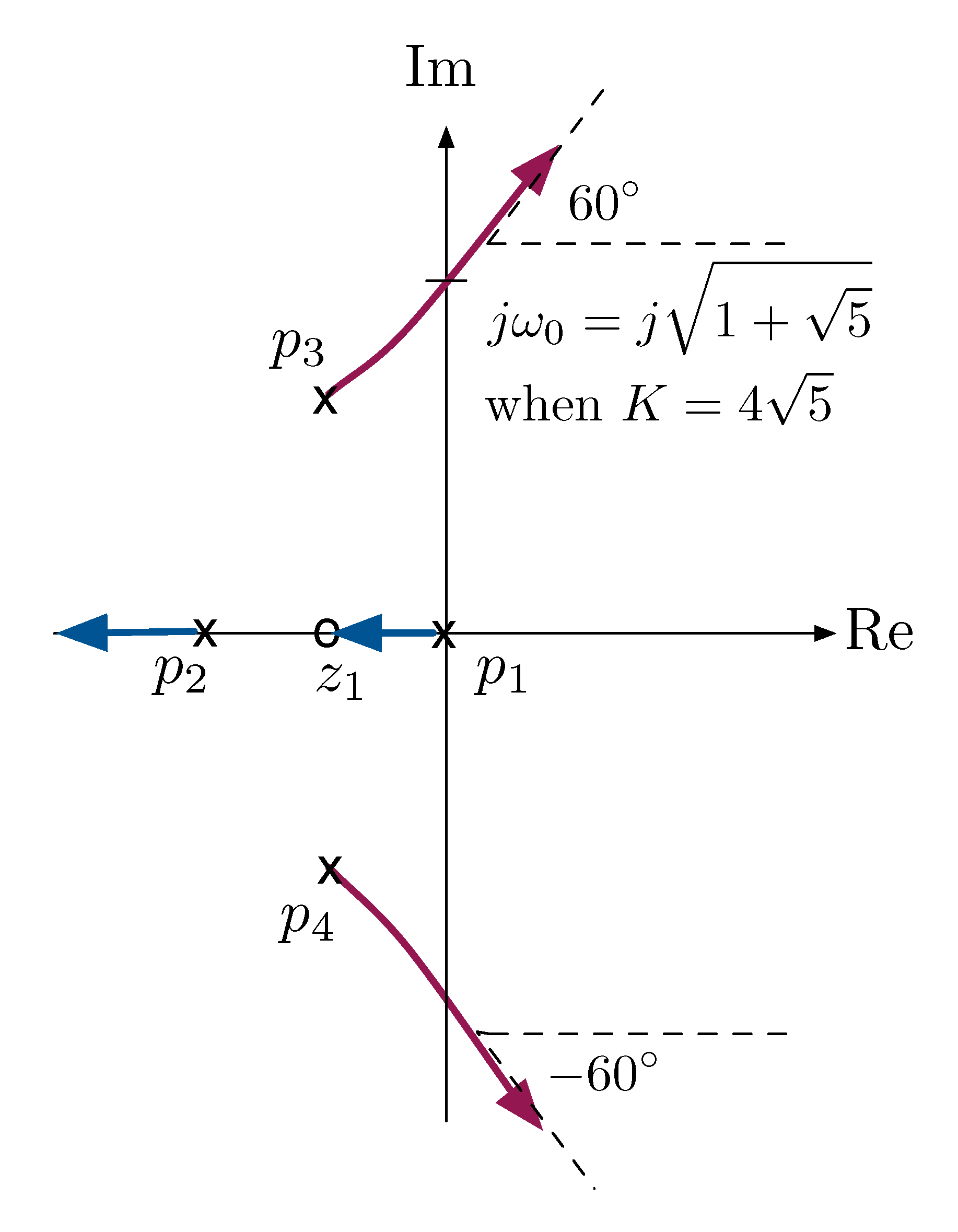
Figure 4: Root locus for Example 2
Using Root to Select Parameter Values
In Lab 5, we will need to select the value of gain \(K\) that corresponds to a desired pole on the root locus.
One way of doing it is
\begin{align*} L(s) &= - \frac{1}{K}, \text{ a negative real number.} \\ \implies K &=-\frac{1}{L(s)} \\ &= \frac{1}{|L(s)|}. \\ \end{align*}Then
\begin{align*} L(s) &= \frac{(s-z_1)\cdots(s-z_m)}{(s-p_1)\cdots(s-p_n)} \\ \implies K &= \frac{1}{|L(s)|} = \frac{|s-p_1| \cdots |s-p_n|}{|s-z_1| \cdots |s-z_m|}. \end{align*}Control Design Using Root Locus
Case study: Double Integrator with transfer function \(G(s) = \dfrac{1}{s^2}\)
Consider the transfer function \(G(s) = \frac{1}{s^2}\). We want to ensure stability of the closed loop system while at the same time we want to meet time response specs.
Double Integrator with P-Control
First consider proportional control only as in Figure 5.

Figure 5: Double integrator with P-control
The closed-loop transfer function is
\[ \dfrac{\frac{K}{s^2}}{1+\frac{K}{s^2}} = \dfrac{K}{s^2 + K}. \]
So characteristic equation is
\[ s^2 + K = 0. \]
We have the closed-loop poles \(s = \pm \sqrt{K}j\) as in Figure 6.
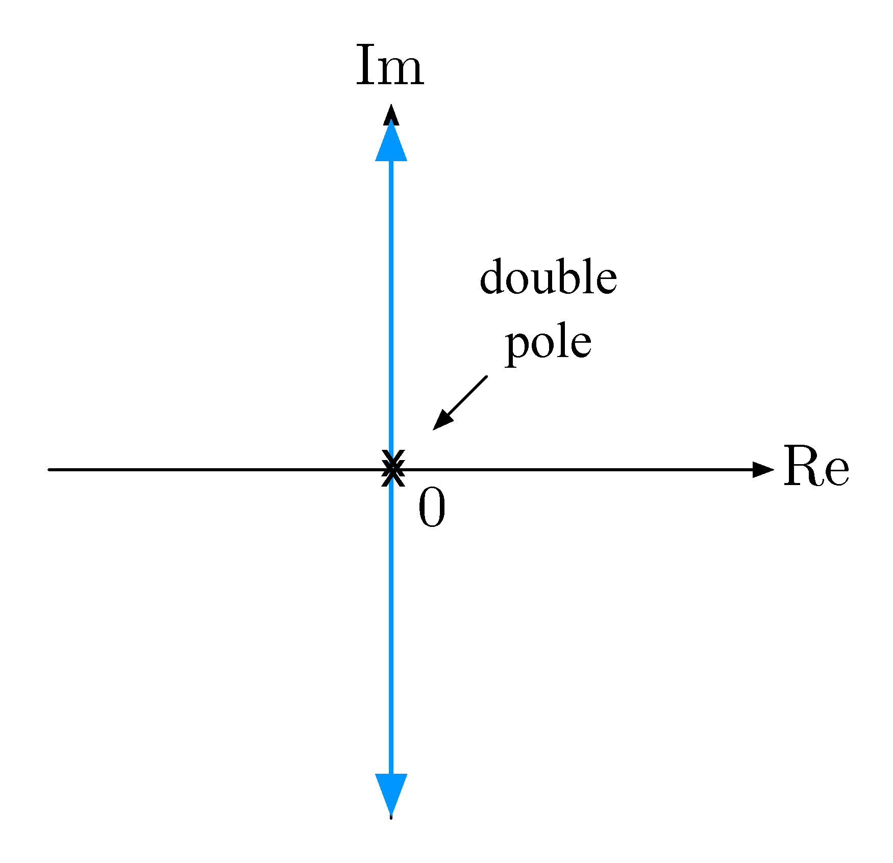
Figure 6: Root locus for double integrator with P-control
This confirms what we already knew—P-control alone does not deliver stability.
Double Integrator with PD-Control
Next consider PD-Control as shown in Figure 7.

Figure 7: Double integrator with PD-control
The characteristic equation in this case is
\begin{align*} 1 + \underbrace{(K_{\rm P} + K_{\rm D}s)}_{G_c(s)} \cdot \underbrace{\frac{1}{s^2}}_{G_p(s)} &= 0, \\ s^2 + K_{\rm D}s + K_{\rm P} &= 0. \end{align*}To use the Root Locus Method, we convert it into the Evans form
\[1 + KL(s) = 0,\]
where
\[L(s) = \dfrac{b(s)}{a(s)} = \dfrac{s^m + b_1 s^{m-1} + \cdots}{s^n + a_1 s^{n-1} + \cdots}.\]
By
\[ 1 + (K_{\rm P} + K_{\rm D}s)\frac{1}{s^2} = 1 + K_{\rm D} \cdot \frac{s + K_{\rm P}/K_{\rm D}}{s^2}, \]
choose \(K = K_{\rm D}\) as the varying parameter, further assuming \(K_{\rm P}/K_{\rm D}\) is fixed, say it is \(1\), then
\[L(s) = \frac{s + K_{\rm P}/K_{\rm D}}{s^2}.\]
The characteristic equation becomes \[1 + K\cdot \dfrac{s + 1}{s^2} = 0.\]
We can write out the roots explicitly
\begin{align*} s^2 + Ks + K = 0 \implies s_{1,2} = \frac{-K \pm \sqrt{K^2 - 4K}}{2}. \end{align*}But let’s actually draw the root locus using the Rules A — F.
- Rule A says there are 2 branches;
- Rule B says both branches start at \(s=0\);
- Rule C says one ends at \(z_1 = -1\), the other at \(\infty\);
- Rule D says one branch will go off to \(-\infty\) on the real axis;
- Rule E says asymptote angles at \(180^\circ\);
- Rule F says no $jω$-crossings except for \(s=p_1=p_2 = 0\).
The root locus is shown in Figure 8.
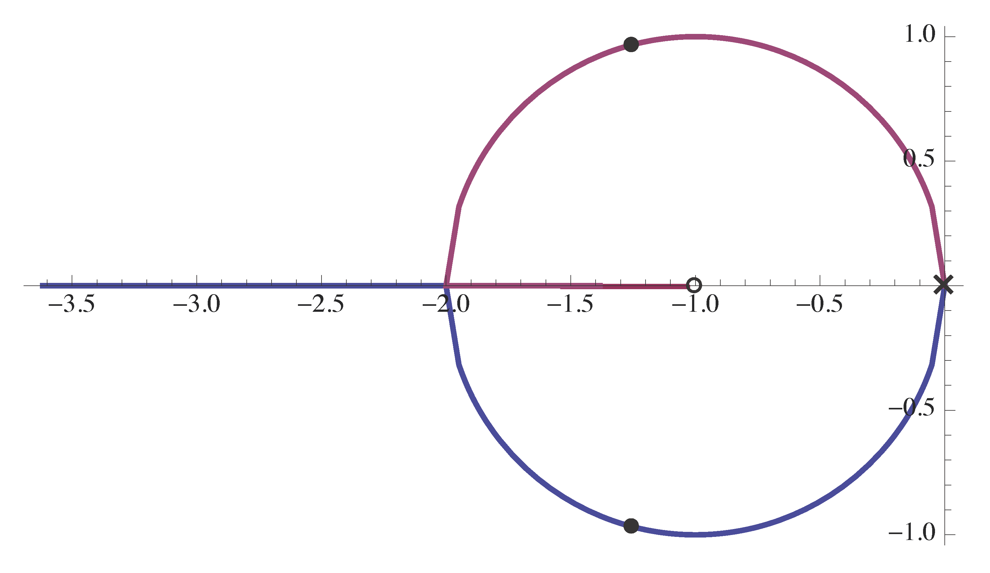
Figure 8: Root locus for double integrator with PD-control
From Figure 8 regarding stabilization, we conclude that
- all closed-loop poles are in the Left Half Plane; (We already knew this from Routh test, but now it is visualized.)
- we may have nice damping, so our design can meet reasonable specs.
Therefore the effect of D-control was to introduce an open-loop zero to \(L(s)\) in the Left Half Plane, and this zero “pulled” the root locus into LHP, thus stabilizing the system.
Approximate PD Using Dynamic Compensation
From the above discussion, we know we can use root locus to visualize the effect of adding D-control: add a Left Half Plane zero, it will pull the closed-loop poles into LHP; hence stabilization.
However, we already know that PD control is not physically realizable since its lack of causality.
Dynamic compensation deals with controllers more general than just P-control, but implementable by causal systems of the form
\begin{align*} \dot{z} &= Az + Be \\ u &= Cz + De. \end{align*}
Figure 9: Dynamic compensation
Any proper transfer function is admissible since they are causal.
Recall from Lecture 9, we can approximate the D-control component \(K_{\rm D}s\) by
\begin{align*} K_{\rm D}\frac{ps}{s+p} \longrightarrow K_{\rm D}s \text{ as } p \to \infty. \end{align*}In the above approximation, \(-p\) is the pole of the controller.
We replace the PD controller \(K_{\rm P} + K_{\rm D}s\) by
\begin{align*} K(s) = K_{\rm P} + K_{\rm D}\frac{ps}{s+p}. \end{align*}Therefore the characteristic equation becomes
\[1 + \left( K_{\rm P} + K_{\rm D}\dfrac{ps}{s+p} \right) G(s) = 0.\]
Matching the Evans form for root locus, we rewrite the PD controller
\begin{align*} K_{\rm P} + K_{\rm D}\frac{ps}{s+p} &= \frac{(K_{\rm P} + pK_{\rm D})s + pK_{\rm P}}{s+p} \\ &= (K_{\rm P} + pK_{\rm D}) \cdot \frac{s + \frac{pK_{\rm P}}{K_{\rm P}+p K_{\rm D}}}{s+p}. \end{align*}Now the PD controller is in the form of \(K \cdot \frac{s+z}{s+p}\), where
- the parameter \(K = K_{\rm P} + pK_{\rm D}\) is a combination of P-control gain, D-control gain, and \(p\);
- the controller has an open-loop zero at \(-z = -\frac{pK_{\rm P}}{K}\).
Recall the example of double integrator, apply dynamic compensation as in Figure 10.

Figure 10: Dynamic compensation for double integrator
The characteristic equation in this dynamic compensation scenario is
\[ 1 + K \cdot \underbrace{\dfrac{s+z}{s+p} \cdot \dfrac{1}{s^2}}_{:=L(s)} = 1 + KL(s) = 0. \]
Notice that \(L(s)\) is not the open-loop transfer function; it comes from the forward gain (equivalent open-loop transfer function) shaped by the controller acting on the plant.