ECE 486 Control Systems
Lecture 10
Root Locus Method
Last time we finished our discussion of PID control and we also talked about system type and its relation to tracking error when reference signal is a polynomial input.
Today, we will start a new chapter on Root Locus method. The Root Locus method is a way of visualizing the locations of closed-loop poles of a given system as some system parameter is varied. It was invented by Walter R. Evans around 1948.
Recall what we have done so for in this course.
- Modeling: We can use differential equations, transfer functions or state space models to describe system dynamics, characterize its output; we can use block diagrams to visualize system dynamics and output.
- Analysis: Based on system closed-loop transfer function, we can compute its response to step input. We can further run Routh-Hurwitz stability test.
- Design: Once we have some decent understanding of system dynamics, we can start control design. For example, we used Routh-Hurwitz criterion as a design tool for a simple system in Example 4, Lecture 7.
We shall focus on design from now on.
Consider unity feedback configuration in Figure 1,

Figure 1: Block diagram for Evans Root Locus method
where
- \(K\) is a constant gain and
- \(L(s) = \dfrac{b(s)}{a(s)}\) is a rational function for some polynomials \(a(s)\) and \(b(s)\).
The system closed-loop transfer function is \(\dfrac{Y}{R}(s) = \dfrac{KL(s)}{1+KL(s)}\), where \(L(s) = \dfrac{b(s)}{a(s)}\).
To compute closed loop poles, we extract characteristic polynomial from closed loop transfer function \(\frac{Y}{R}(s)\) and set it as \(0\), hence we solve for \(s\) according to characteristic equation \(1 + KL(s) = 0\).
\[ 1 + KL(s) = 0 \iff L(s) = -\frac{1}{K}. \\ \]
On the other hand,
\begin{align*} & 1 + KL(s) = 0 \tag{1} \label{d10_eq1} \\ \iff & 1 + \frac{Kb(s)}{a(s)} = 0 \\ \iff & \underbrace{a(s) + Kb(s)}_{\text{characteristic} \atop \text{polynomial}} = 0. \qquad \text{(characteristic equation)} \end{align*}Remark: We changed notation for plant block from
\[ H(s) \text{ or } G(s) = \frac{q(s)}{p(s)} \]
to
\[ L(s) = \frac{b(s)}{a(s)} \]
in Figure 1. But the Root Locus method is quite general, so \(L(s)\) is not necessarily the plant transfer function, and \(K\) is not necessary feedback gain. \(K\) could be any varying parameter of interest. \(L(s)\) and \(K\) may be related to plant transfer function and feedback gain through some transformation. As long as we can represent the poles of the closed-loop transfer function as roots of the equation \(1 + KL(s) = 0\) for some choice of \(K\) and \(L(s)\), we can apply the Root Locus method.
Root Locus and Quantitative Characterization of Stability
Routh test gives us a range of \(K\) to guarantee stability. On top of stability requirement, a further natural question would be, for what values of \(K\) do we best satisfy given design specs? Figure 2 shows the possible pole locations when time domain specifications are constrained as we discussed in Lecture 6.
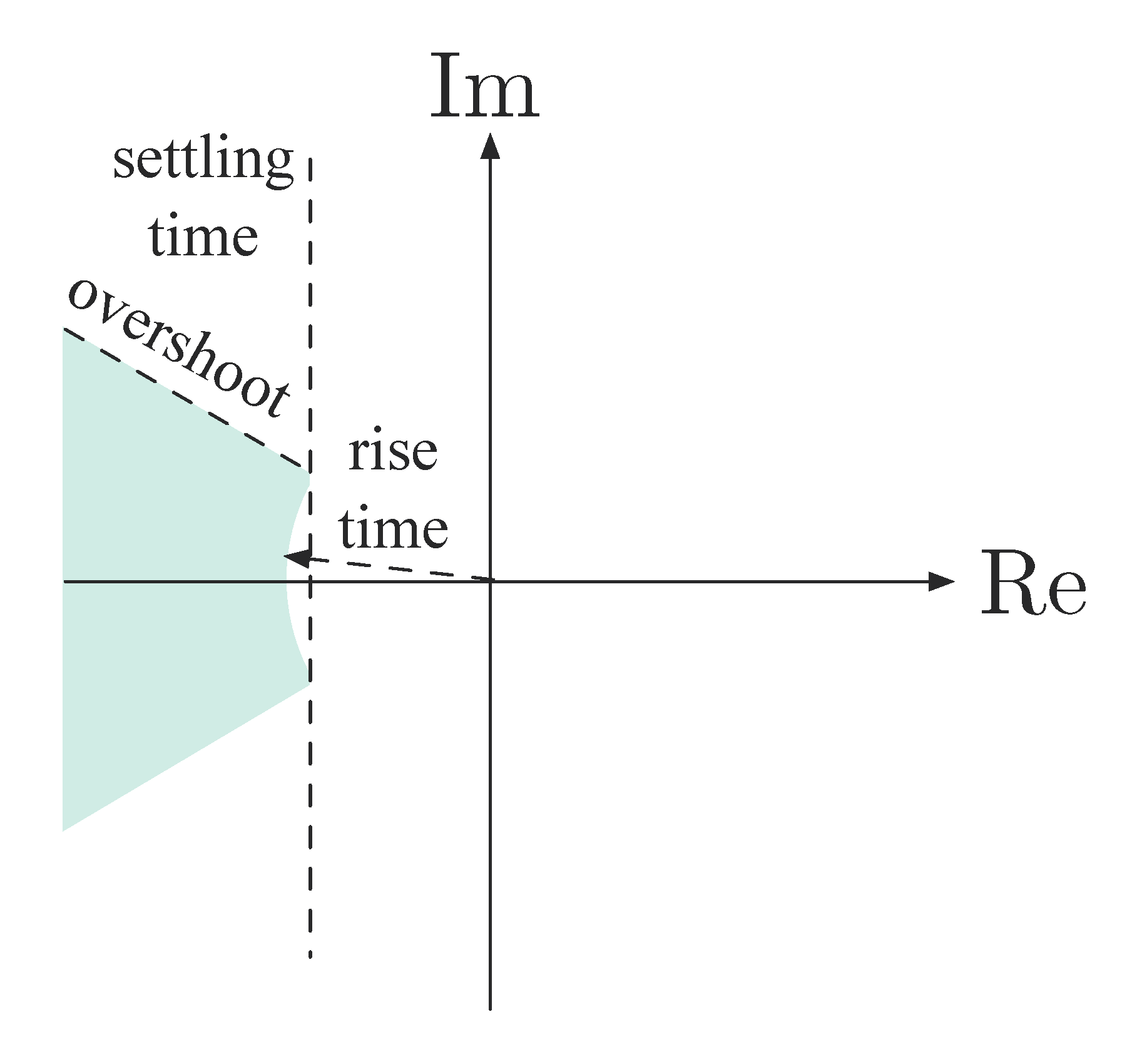
Figure 2: Admissible pole locations with constrained time domain specifications
We note time domain specifications are encoded in closed loop pole locations in Equation \eqref{d10_eq1}. Therefore we define the root locus for \(1+KL(s)\) as the set of all closed-loop poles, i.e., the roots of
\[ 1 + KL(s) = 0 \]
as \(K\) varies from \(0\) to \(\infty\).
Consider Figure 1 with
\begin{align*} L(s) &= \frac{1}{s^2+s} \text{, i.e.,}\\ b(s) &= 1, a(s) = s^2+s \end{align*}as our first example. The characteristic equation \(a(s) + Kb(s) = 0\) becomes
\[ s^2 + s + K = 0. \]
By the quadratic formula, the roots are \[ s_{1,2} = - \dfrac{1\pm \sqrt{1-4K}}{2} = - \dfrac{1}{2} \pm \dfrac{\sqrt{1-4K}}{2}. \]
When the parameter \(K\) ranges from \(0\) to \(\infty\),
\[ \text{Root locus} = \left\{ - \dfrac{1}{2} \pm \dfrac{\sqrt{1-4K}}{2} : 0 < K < \infty \right\} \subset \CC. \]
Let’s sketch the root locus in the complex plane.
Step 1: Start with \(K=0\), the two roots are \(s_{1,2} = -\frac{1}{2} \pm \frac{1}{2} = -1,0\). They are also open-loop poles since feedback \(K = 0\) brings no change to open loop \(L(s)\). As a start, we have two points in the graph as in Figure 3.
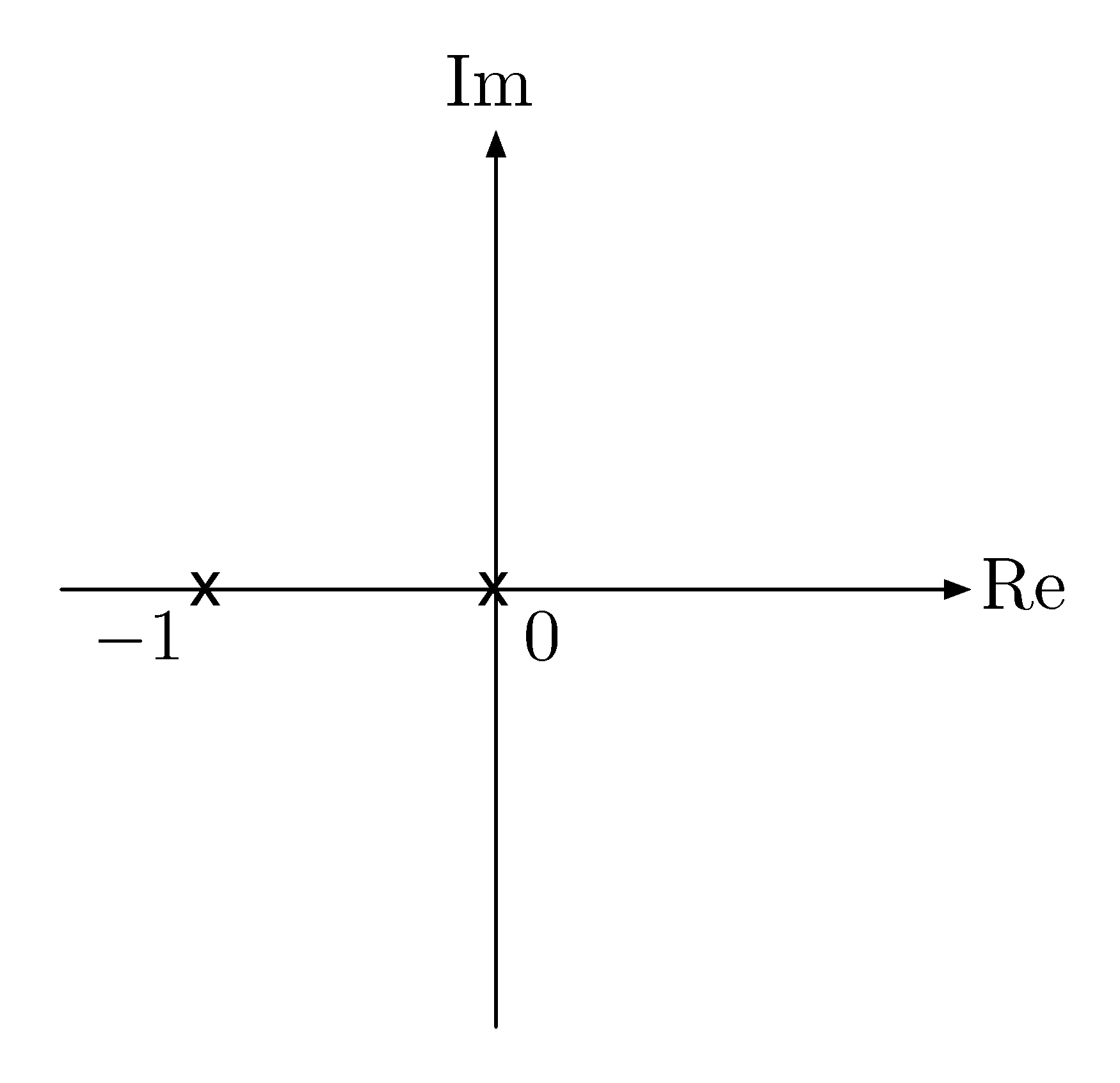
Figure 3: Sketching root locus with \(L(s) = \frac{1}{s^2+s}\), step 1
Step 2: As \(K\) increases from \(0\), the poles start to move.
- (a) When \(1 - 4K \geq 0\), i.e., \(0 < K \leq \frac{1}4\), the poles are two real poles; they stay on the real axis as in Figure 4.
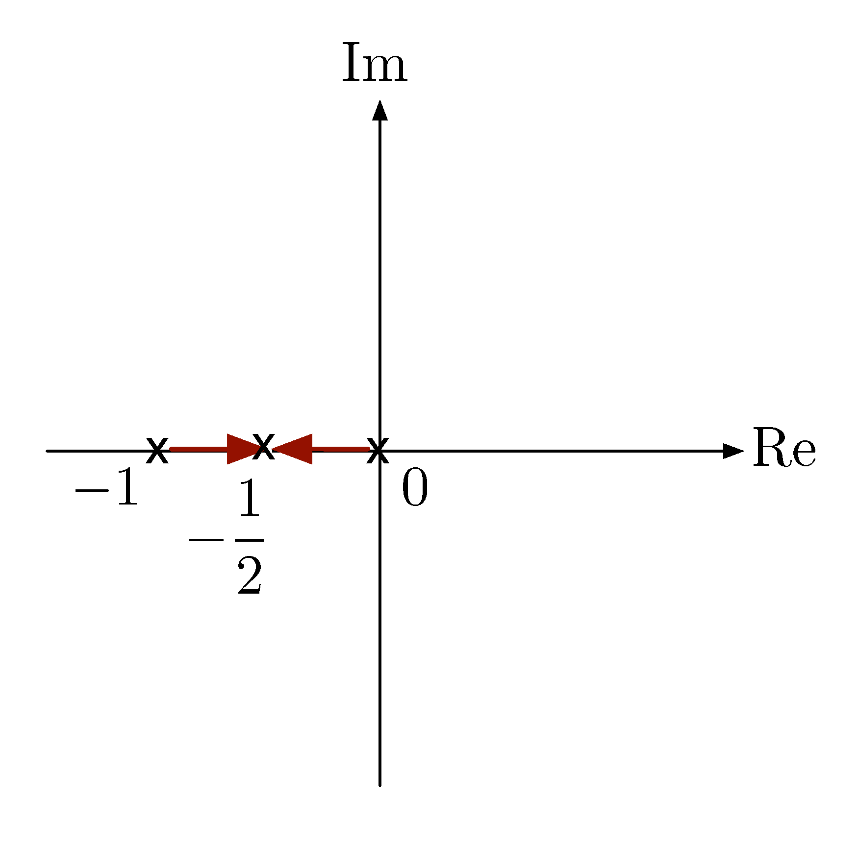
Figure 4: Sketching root locus with \(L(s) = \frac{1}{s^2+s}\), step 2 (a)
- (b) When \(1 - 4K < 0\), i.e., $ K > \frac{1}4$, the poles are two complex poles with constant real part \({\rm Re}(s) = -\frac{1}2\) as in Figure 5.
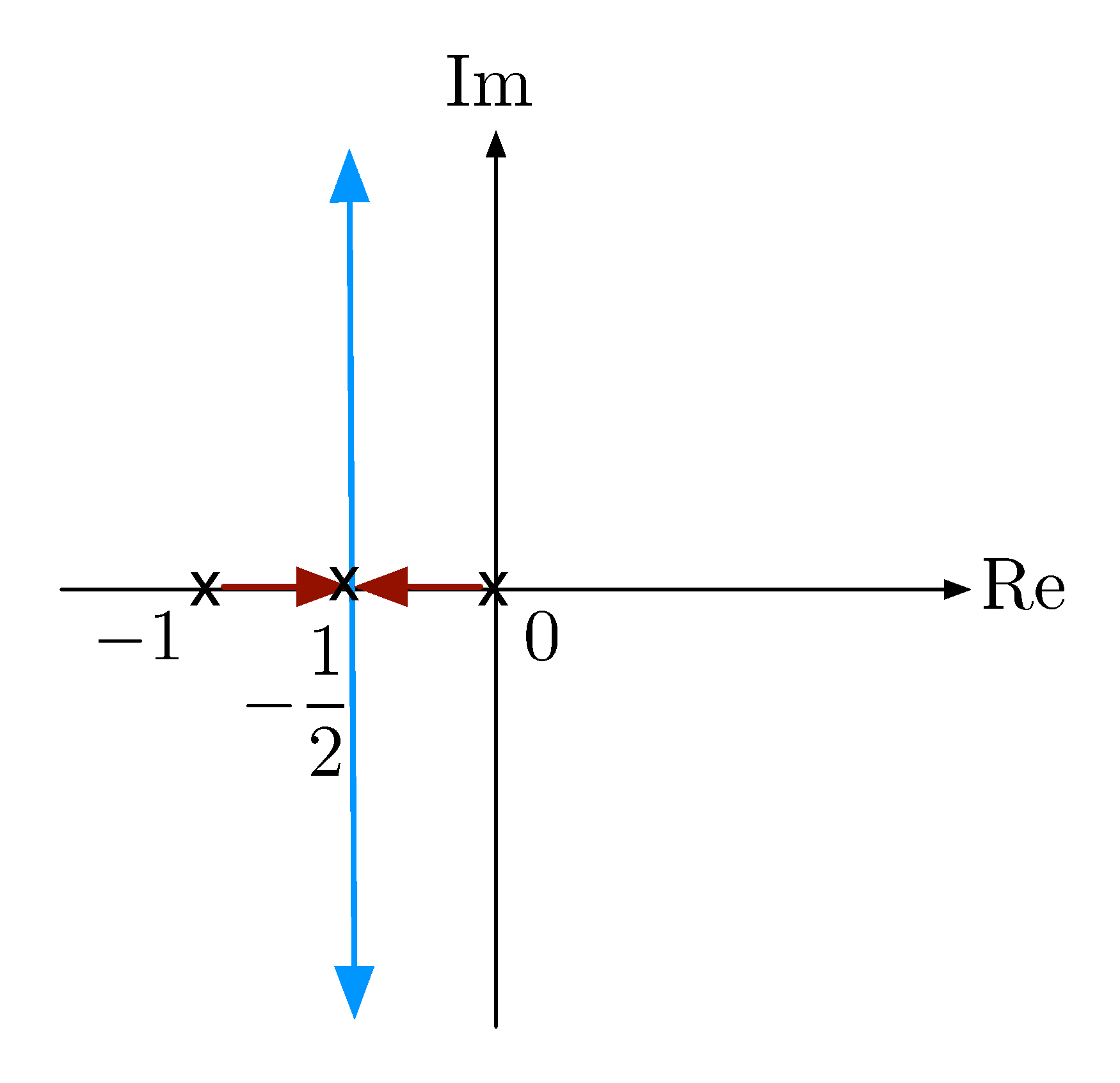
Figure 5: Sketching root locus with \(L(s) = \frac{1}{s^2+s}\), step 2 (b)
The point \(s=-\frac{1}2\) is the point of breakaway of root locus from the real axis.
Recall from Lecture 6 the relationship between time domain specifications and pole locations,
- \(t_s \approx \frac{3}{\sigma}\), a quickly settled response requires a large \(\sigma\). Here we have a fixed \({\rm Re} (s) = -\sigma = -\frac{1}{2}\), hence \(t_s \approx 6\).
- \(t_r \approx \frac{1.8}{\omega_n}\), a fast rising response requires a large \(\omega_n\), hence a large \(K\).
\(M_p\) is associated with the boundary of the shaded cone as in Figure 6. A system response with small overshoot requires poles be inside the shaded region. From the figure, \(K\) shall remain small.
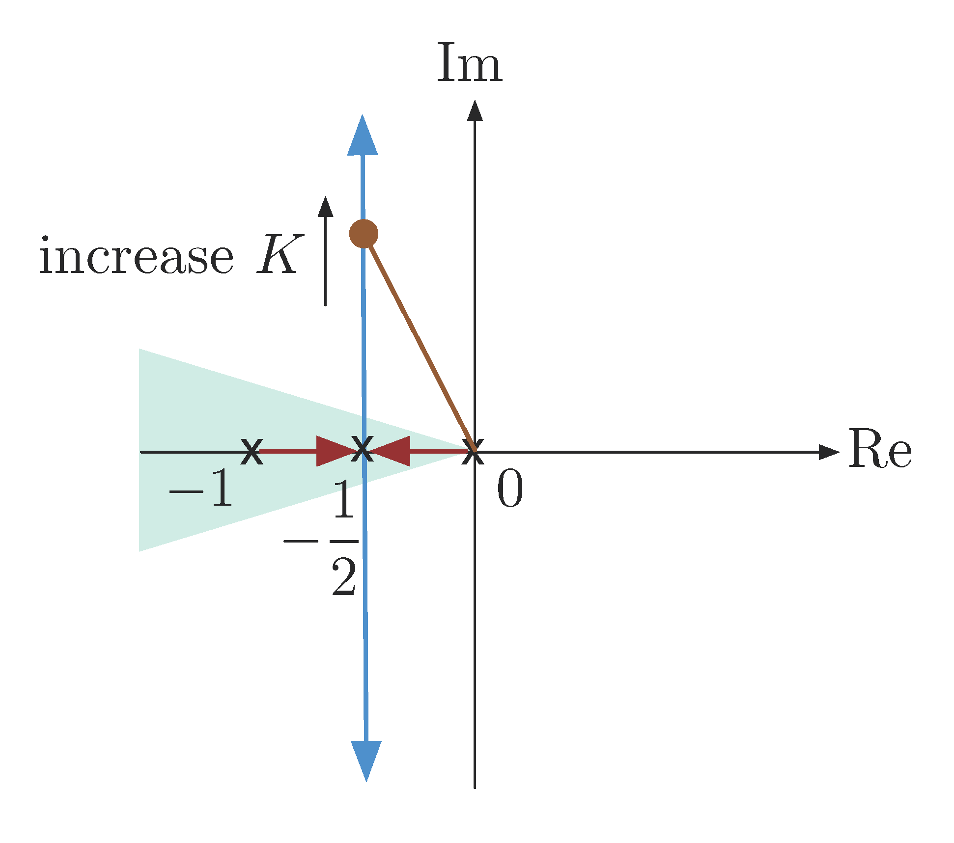
Figure 6: Overlaid root locus and admissible pole locations with constrained time domain specifications, where \(L(s) = \frac{1}{s^2+s}\)
Thus, from this first example, we saw the root locus helps us visualize the trade-off between all the specs in terms of \(K\). However, for systems with order greater than \(2\), there will generally be no direct formula for the closed-loop poles as a function of \(K\). This is why we want to develop simple rules for sketching approximate root locus in the general case.
Equivalent Characterization of Root Locus: Phase Condition
Recall our original definition, the root locus for \(1+KL(s)\) is the set of all closed-loop poles, i.e., the roots of \[ 1 + KL(s) = 0, \]
as \(K\) varies from \(0\) to \(\infty\).
A point \(s \in \CC\) on the complex plane is on the root locus if and only if
\[ \tag{2} \label{d10_eq2} L(s) = \underbrace{-\dfrac{1}{K}}_{\text{negative and real}} \text{ for some $K > 0$}. \]
Equation \eqref{d10_eq2} says its right hand side is real and negative since \(K\) is real and positive. This gives us an equivalent characterization of root locus
The phase condition of root locus: The root locus of \(1 + KL(s)\) is the set of all \(s \in \CC\), such that \(\angle L(s) = \pm 180^\circ\), i.e., \(L(s)\) is real and negative.
Rules for Sketching Root Loci (Rules A — D)
There are six rules for sketching root loci. These rules are mainly qualitative, and their purpose is to give intuition about impact of poles and zeros on performance.
These rules are
- Rule A — number of branches
- Rule B — start points
- Rule C — end points
- Rule D — real locus
- Rule E — asymptotes
- Rule F — $jω$-crossings
We will cover mostly Rules A — C (and a bit of D) in this lecture.
Rule A: Number of Branches
Let \(L(s) = \frac{b(s)}{a(s)}\). Write out the characteristic equation in \eqref{d10_eq1},
\begin{align*} &1 + K\frac{b(s)}{a(s)} = 1 + K \frac{s^m + b_1 s^{m-1} + \ldots + b_{m-1}s + b_m}{s^n + a_1 s^{n-1} + \ldots + a_{n-1}s + a_n} = 0 \\ \iff & (s^n + a_1 s^{n-1} + \ldots + a_{n-1}s + a_n) + K(s^m + b_1 s^{m-1} + \ldots + b_{m-1}s + b_m) = 0. \end{align*}But \(\deg(a) = n \ge m = \deg(b)\) (\(L(s)\) is proper), the polynomial \(a(s) + Kb(s)\) has degree \(n\). Therefore, the characteristic equation has \(n\) not necessarily distinct roots, some of which may be repeated. As we vary \(K\), these \(n\) solutions also vary to form \(n\) branches.
Note: The reason why both polynomials \(a(s)\) and \(b(s)\) can be monic in \(L(s) = \frac{b(s)}{a(s)}\) is that suppose we use the most general \(L(s)\),
\[L(s) = \frac{B(1\cdot s^m + \cdots)}{A(1\cdot s^n + \cdots)} \]
with \(A, B\) constants. Then when we study the root locus of \(1 + K L(s) = 0\), ranging \(K\) from \(0\) to \(\infty\) is the same as ranging \(K\cdot \frac{B}A\), i.e., scaling the range \((0, \infty)\) by a constant will not affect the fact that all the cases of interest have been covered when we range \(K\) from \(0\) to \(\infty\).
Rule A: The number of branches of root locus is equal to the degree of the denominator of \(L(s)\), i.e., \[ \#\text{branches of root locus} = \deg(a(s)). \]
Rule B: Start Points
The locus starts from \(K = 0\). What happens near \(K = 0\)?
By \(a(s) + Kb(s) = 0\), if \(K \to 0\), then \(a(s) = - Kb(s) \to 0\). (Why? Hint: \(b(s)\) is bounded except for \(s = \infty\) since \(b(s)\) is a polynomial.)
Therefore either
- \(s\) is close to a root of \(a(s) = 0\), or equivalently
- \(s\) is close to a pole of \(L(s)\).
Caution: The reasoning here essentially is saying when \(K\) is small, the coefficients of polynomial \(a(s) + Kb(s)\) differ term-wise from the coefficients of the polynomial \(a(s)\) by some tiny bit, therefore the two sets of roots must be similar. It is false however in numerical analysis, see the examples given by Wilkinson.
A better argument would be to use the fact that the roots of a polynomial with complex coefficients (hence including the case of real coefficients) continuously depend on this polynomial’s coefficients. See properties of polynomial roots on Wikipedia.
Rule B: Branches of root locus start at open-loop poles.
Rule C: End Points
We considered one end point of the range of \(K \in (0, \infty)\) in Rule B. Now let’s consider the other end point at infinity \(K \to \infty\). Since \(K\) is not zero, we can divide out \(K\) on both sides,
\begin{align*} 0 &= a(s) + Kb(s), \\ b(s) &= -\frac{1}{K}a(s). \end{align*}As \(K \to \infty\), \(b(s) \to 0\) (since \(a(s)\) is finite), i.e., \(s\) is around some root of \(b(s)\).
- branches end at the roots of \(b(s) = 0\), or equivalently
- branches end at zeros of \(L(s)\).
Rule C: Branches of root locus end at open-loop zeros.
Note if \(n > m\) when \(L(s)\) is strictly proper, we have \(n\) branches, but only \(m\) zeros. This is not a problem since the remaining \(n-m\) branches go off to infinity; they end at “zeros at infinity”.
Example 1: Consider the PD control of an unstable second order plant that we used last time,

Figure 7: PD control of unstable \(G(s) = \frac{1}{s^2 - 1}\)
sketch the root locus by choosing parameter \(K = K_{\rm D}\) with fixed ratio \(\frac{K_{\rm P}}{K_{\rm D}}\).
Solution: In order to get characteristic equation \(1 + KL(s) = 0\), we need to compute the closed loop transfer function \(\frac{Y}{R}(s)\). (But we don’t solve for its roots; we sketch root locus instead.)
\begin{align*} \frac{Y}{R} (s) &= \frac{G_cG_p}{1+G_cG_p} \\ 0 &= 1 + G_c(s)G_p(s) \hspace{3cm} \text{(characteristic equation)} \\ 0 &= 1 + (K_{\rm P} + K_{\rm D}s)\left(\frac{1}{s^2-1}\right). \tag{3} \label{d10_eq3} \end{align*}We will examine the impact of varying \(K = K_{\rm D}\), assuming the ratio \(K_{\rm P}/K_{\rm D}\) fixed. With fixed \(K_{\rm P}/K_{\rm D}\), rewrite the characteristic equation in Evans form,
\begin{align*} 0 &= 1 + \underbrace{K_{\rm D}}_{K}\left( s + \frac{K_{\rm P}}{K_{\rm D}}\right)\left(\frac{1}{s^2-1}\right) \\ &= 1 + K \underbrace{\frac{s+ \frac{K_{\rm P}}{K_{\rm D}}}{s^2-1}}_{L(s)}, \end{align*}where \(L(s) = \frac{s - z_1}{s^2-1}\) with zero at \(s = z_1 = - \frac{K_{\rm P}}{K_{\rm D}} < 0\).
We apply Rules A — C to \[ L(s) = \frac{s-z_1}{s^2-1}. \]
- Rule A: The degree of the denominator \(a(s)\) of \(L(s) = \frac{b(s)}{a(s)}\) is \(2\), thus there are two branches.
- Rule B: Root locus branches start at open-loop poles, i.e, the roots of \(a(s) = s^2 - 1\), \(s = \pm 1\).
- Rule C: Root locus branches end at open-loop zeros \(s = z_1, - \infty\). (We will see why \(-\infty\) later.)
So the root locus will look something like this,
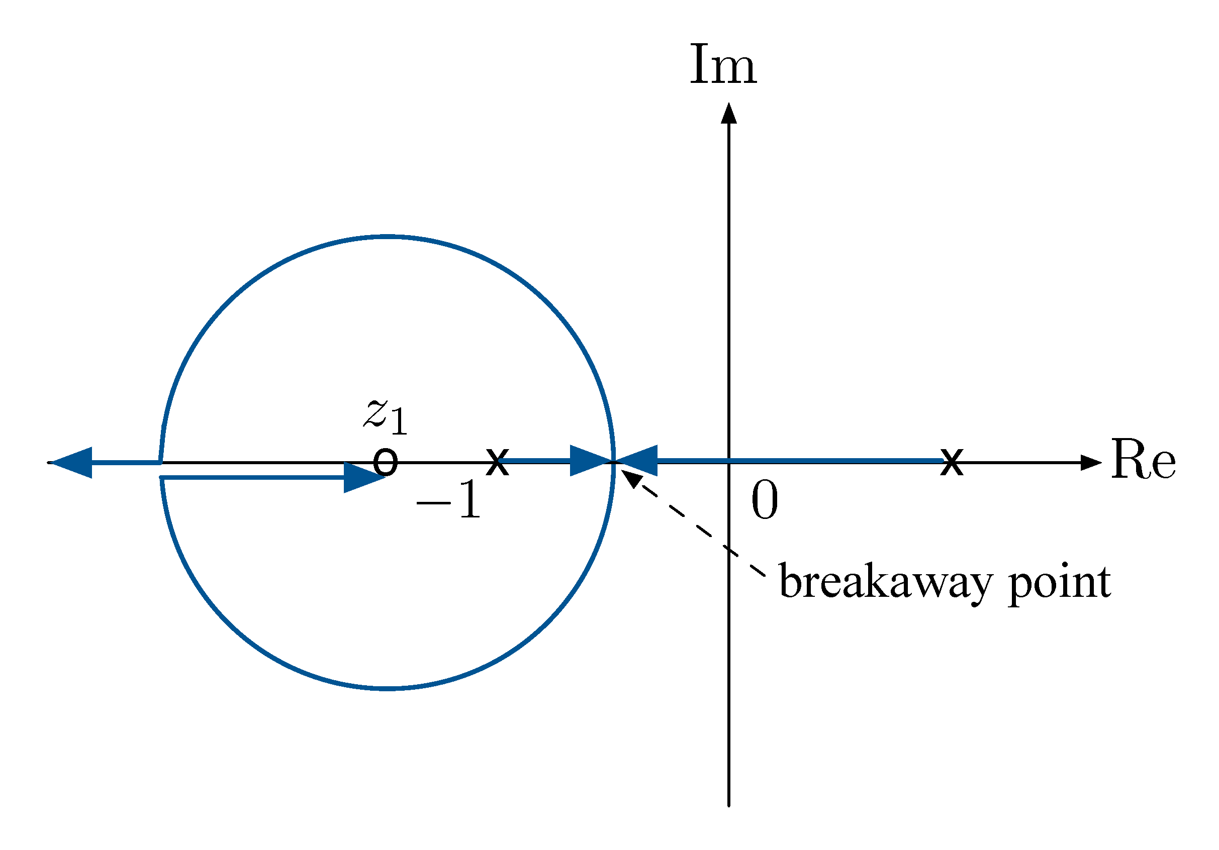
Figure 8: Root locus of \(L(s) = \frac{s-z_1}{s^2-1}\)
Why does one of the branches go off to \(-\infty\)? Indeed, solve for roots by quadratic formula
\begin{align*} s^2-1 + K(s-z_1) = 0 &\\ s^2 + Ks - (Kz_1+1) = 0 &\\ \implies s_{1,2} = - \frac{K}{2} \pm \sqrt{\frac{K^2}{4} + Kz_1 + 1} &. \end{align*}We notice \(z_1 < 0\), as \(K \to \infty\), the term under the square root is approximately \(\frac{K^2}4\) but less than that, hence both \(s_{1,2}\) will be negative.
Why is the point \(s=0\) on the root locus? Because we can find a positive \(K > 0\) such that
\begin{align*} 1 + KL(0) &= 0 \\ 1 + Kz_1 &= 0. \end{align*}This \(K = -\frac{1}{z_1} > 0\) does the job.
What’s the relation to time response specifications? For concreteness, let’s run a numerical example. Let \(\frac{K_{\rm P}}{K_{\rm D}} = -z_1 = 2\) and \(K = K_{\rm D} = 5\). This implies \(K_{\rm P} = 10\).
The characteristic equation in Equation \eqref{d10_eq3} becomes
\begin{align*} 1 + 5 \left( \frac{s+2}{s^2-1}\right) &= 0 \\ \iff s^2 + 5s + 9 &= 0. \end{align*}Matching the coefficients of prototype second order transfer function, we get
\begin{align*} \omega^2_n = 9 &\implies \omega_n = 3, \\ 2\zeta\omega_n = 5 &\implies \zeta = \frac{5}6. \end{align*}Moral of Example 1:
- When zeros are in Left Half Plane, high gain can be used to stabilize the system although one must worry about zeros at infinity.
- If there are zeros in Right Half Plane, high gain is always disastrous since root locus would end at a RHP zero, i.e., closed loop unstable.
- PD control is effective for stabilization because it introduces a zero in Left Half Plane.
But Rules A — C cannot tell the whole story. How do we know which way the branches go, and which pole corresponds to which zero? We need more rules. (Rules D — F)
Example 2: In this example, let’s consider the root locus with \[L(s) = \dfrac{s+1}{s(s+2)\big((s+1)^2+1\big)}.\]
Solution: The equivalent open loop transfer function \(L(s)\) is given and we note
- By Rule A, the degree of its denominator is \(4\), hence the root locus has four branches.
- By Rule B, its branches start at open-loop poles \(s = 0\), \(s=-2\), and \(s=-1 \pm j\).
- By Rule C, one of its branches ends at open-loop zeros \(s = -1\); three other branches end at \(\pm\infty\) because the degree of its numerator is \(1\).
As a start, we can mark down the poles and zeros that are on the root locus at the moment.
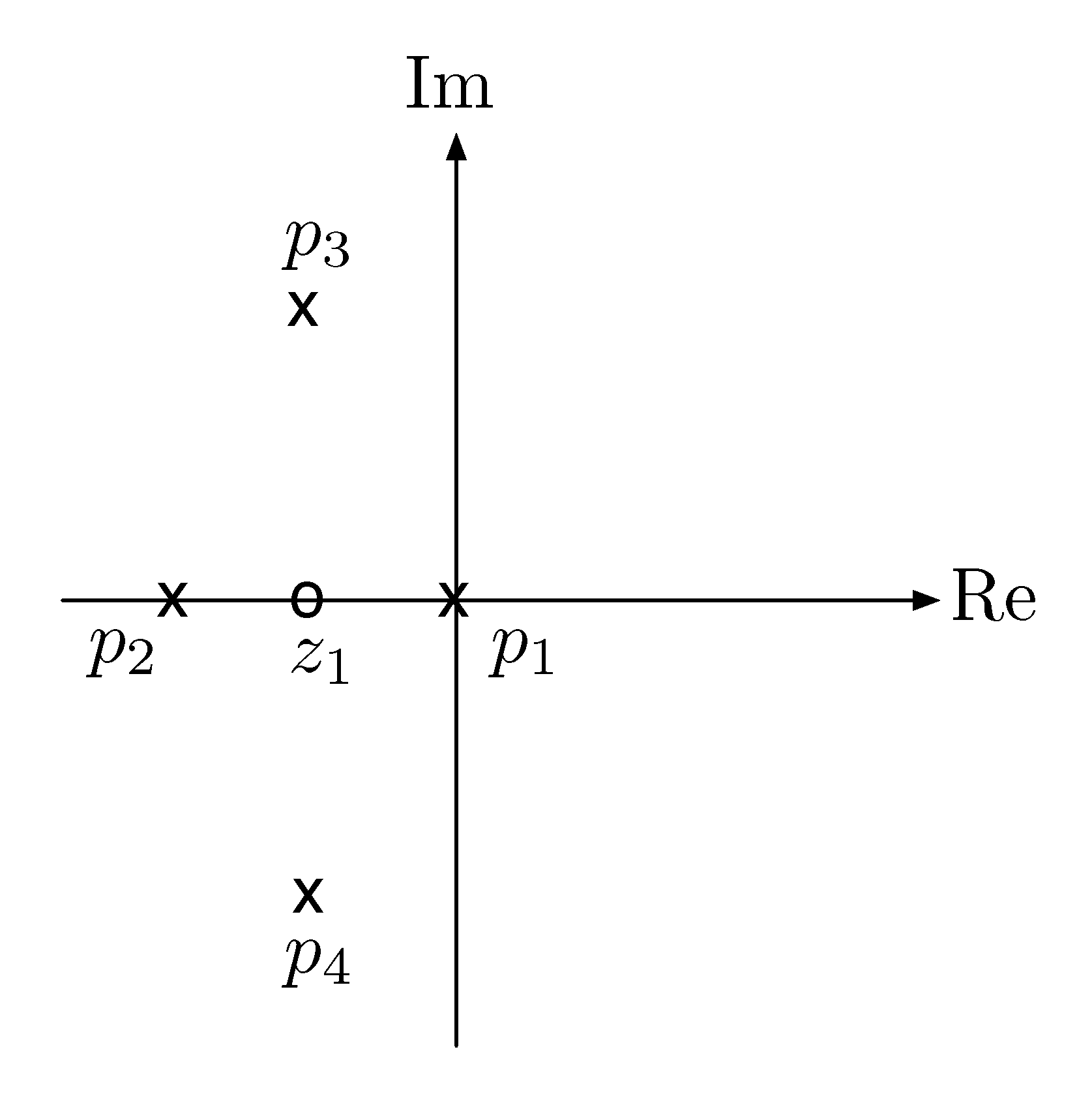
Figure 9: Root locus of $L(s) = \frac{s+1}{s(s+2)\big( (s+1)^2+1 \big)} $, step 1.
We will leave here since we need three more rules to complete the picture.
- Rule D: real locus
- Rule E: asymptotes
- Rule F: $jω$-crossings
Remark: Rules D and E are both based on the fact that \[ 1 + KL(s) = 0 \text{ for some $K > 0$} \quad \iff \quad L(s) < 0. \]
Rule D: Real Locus
The branches of the RL start at the open-loop poles. We ask the question which way do they go, left or right?
Recall the phase condition \[ 1 + KL(s) = 0 \iff \angle L(s) = 180^\circ \] for a positive \(K\). But the angle of \(L(s) = \frac{b(s)}{a(s)}\) is
\begin{align*} \angle L(s) &= \angle \frac{b(s)}{a(s)} \\ &= \angle \frac{(s-z_1) (s-z_2) \cdots (s-z_m)}{(s-p_1)(s-p_2)\cdots(s-p_n)} \\ &= \sum^m_{i=1}\angle (s-z_i) - \sum^n_{j=1}\angle (s-p_j). \hspace{3cm} \text{(by De Moivre's formula)} \end{align*}
This angles sum must be \(\pm 180^\circ\) for any \(s\) that lies on the root
locus. Note again, the form \(L(s)\) assumes here is zero-pole form, which
relies on the fact that both \(a(s)\) and \(b(s)\) are monic. One associated
matlab command is zero-pole-gain zpk().
Now we try some test points as shown in Figure 10.
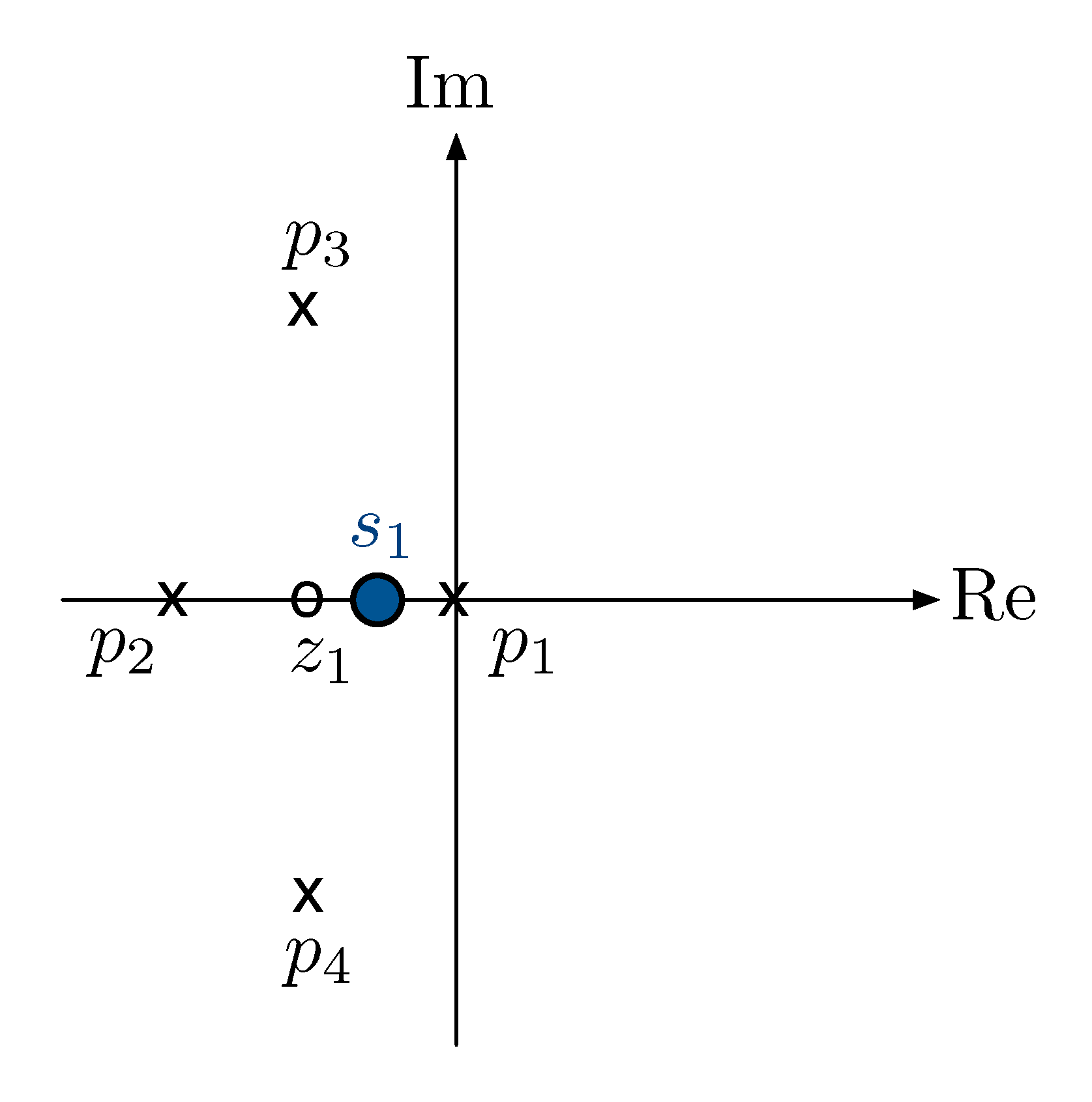
Figure 10: Testing real locus, trial 1
Check angles sum,
\begin{align*} &\angle (s_1 - z_1) - \left[ \angle(s_1-p_1) + \angle (s_1 - p_2) + \angle(s_1 - p_3) + \angle(s_1 - p_4)\right] \\ & = 0^\circ - \left[180^\circ + 0^\circ + 0^\circ\right] \\ & = - 180^\circ . \end{align*}We conclude \(s_1\) in Figure 10 is on the root locus.
Similarly if we continue to test more points
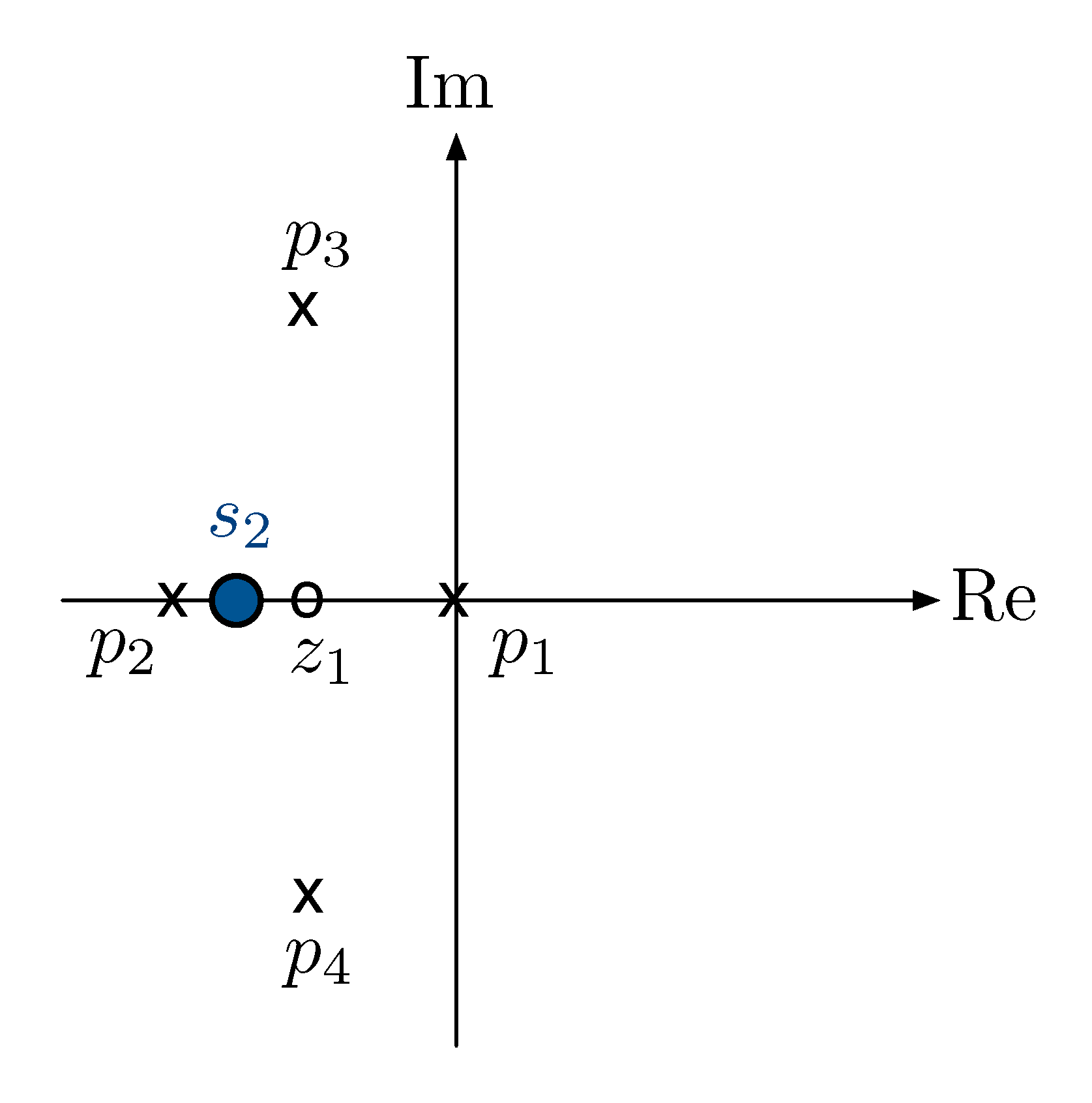
Figure 11: Testing real locus, trial 2
Check angles sum,
\begin{align*} &\angle (s_2 - z_1) - \left[ \angle(s_2-p_1) + \angle (s_2 - p_2) + \angle(s_2 - p_3) + \angle(s_2 - p_4)\right] \\ & = 180^\circ - \left[180^\circ + 0^\circ + 0^\circ\right] \\ & = 0^\circ \neq \pm 180^\circ. \end{align*}We conclude \(s_2\) in Figure 11 is not on the root locus.
Rule D: If \(s\) is real, then it is on the root locus of \(1 + KL(s)\) if and only if there are an odd number of real open-loop poles and zeros to the right of \(s\).
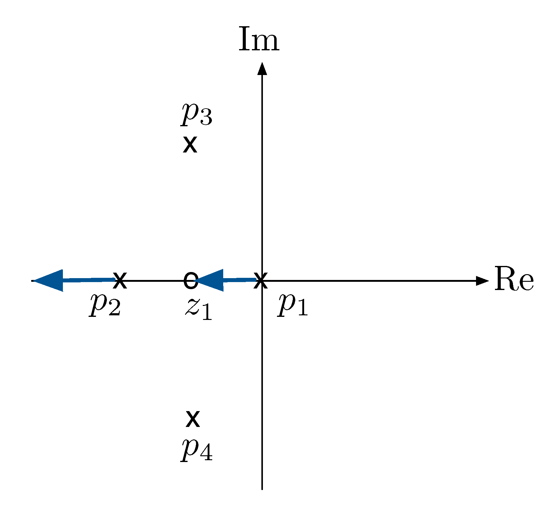
Figure 12: Root locus, Rule D
Rules E and F will be discussed next time, and we shall complete Example 2 then.