Lecture 15

Reading material: Chapter 12 of CSSB

We finally come to the third and last major thematic portion of the course with this lecture. In this lecture we discuss the basic strategies and theory of analysis of simple mechanical and electrical networks. We start with a review of the basic laws and principles of mechanics.

Mechanical systems

The most studied mechanical system is probably the mass-spring-damper system. Why do we worry so much about mass-spring systems, you may be wondering. We research these systems because they can be used to represent or simplify a wide range of engineering issues. Several of these consist of:

• Solid mechanics systems: small local sections of a material can be modeled as a springs with damping

• Fluid flow: mass-spring models serve as one starting point for deriving the equations of motion for fluids

• Circuits: the next section of the notes will show how many circuit elements share similiarities with mass-spring-damper systems

• Real mass-spring-damper mechanisms: obviously

• Mechanical computers: see for example Voskhod Globus

• Musculo-skeletal systems: actual biological mechanics is often modeled using mass-spring-damper systems

In the sections that follow, we'll first go through a mass spring system's fundamental parts and how to set up the equations. Masses, springs, and dashpots (or dampers) are the three major parts of mass spring systems. The equation(s) of motion for the system are derived using Newton's second law along with the equations for the spring and friction (dashpot) forces. Let's have a look at a really straightforward mass spring system we already have seen before:

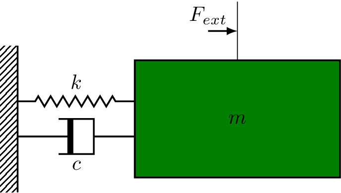
We should already know from PHYS 211 that the force exerted by the spring is in opposition to motion and dependent on the total displacement from its equilibrium position. The spring constant $k$ tells us how much force is generated per unit displacement and thus takes units N/m. On the other hand, the force exerted by the dashpot is proportional the rate of change of displacement, i.e. velocity. Therefore this term is also often called a viscous damper (in relation to viscous liquids like a can of thick paint). Both these forces along with the applied external force are related to the acceleration experienced by the object (by Newton's second law of motion).

$$m \ddot{x} = F_{ext} -kx - c \dot x$$

As a preview of BIOE 420, often this second order system is written as two coupled first order differential equations by the introduction of state variables $z_1=x$ and $z_2 = \dot{z_1}$ which are displacement and velocity respectively as:

Most mechanical systems we will concern ourselves with are different arrangements of the above basic components.

Exercise: Derive the coupled second order ODEs which represent the equations of motion for the following system:

To get (1) above written in the standard second order ODE format we are already familiar with, i.e.

we need to set:

This puts our system in the form that we have examined in detail in the previous lecture - Lecture 14. In particular, there we discussed the how different values of $\zeta$ lead to qualitatively different responses from the system and we examined those responses using a demonstration. Recall that these were the cases of: underdamped, overdamped and critically damped systems.

In this lecture note we further discuss two more qualitatively different responses that can come from such systems which have to do with the relative values of $\omega_n$ and the forcing frequency $\omega$ of the input function $F(\omega)$.

Forced motion means there is some sort of outside force acting on the masses (i.e. motion independent of the spring or damping forces). Let’s modify the above mass-spring system slightly to include a forcing term i.e. something driving the mass that is driven separately from the mass:

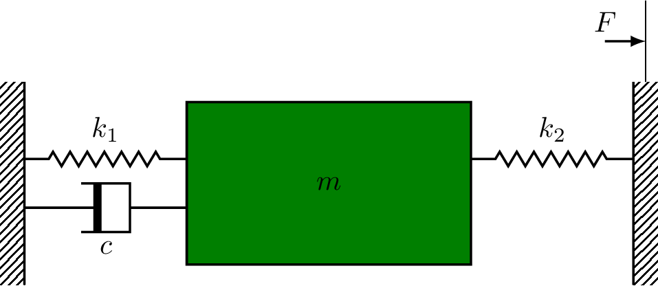
Note that $F$ above can be either a function for force or displacement of the right endpoint.

Exercise: Derive the equations of motion for the above system.

In the following we assume that the reader is familiar with second order differential equations of the inhomogenous type (see MATH 285 syllabus); i.e. with forcing term present. Let the forcing function be sinusoidal with frequency $\omega$. Then we have four cases to discuss:

• When the system is damped (and therefore has a decaying homogeneous solution), a case well discussed in MATH 285 and in last lecture.

• When the system is undamped and its natural frequency $\omega_n$ is very different from the forcing frequency $\omega$.

• When the system is undamped and $\omega \sim \omega_n$.

• When the system is undamped and $\omega = \omega_n$

Damped systems or $\zeta \neq 0$.

Quite simply, in the first instance with damping, we know that the homogeneous solution will be a decaying sinusoid, and we know that the specific solution will be a sine/cosine from the method of undetermined coefficients. The homogeneous solution is referred to as the transient solution since it degrades/fades with time. The particular solution is known as the steady-state solution since it consists just of a sine or cosine that never ends.

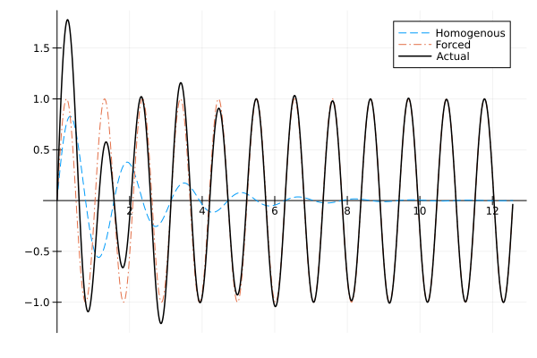
In general, you should picture the solution's appearance as $t\to \infty$ when you hear the term "steady state solution". We have already examined what happens with different values of $\zeta$ the damping coefficient and so we don't repeat it here.

Undamped systems or $\zeta = 0$.

The cases of real interest for this lecture note are what happens without damping in the presence of a forcing function.

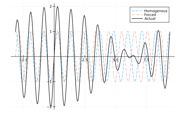
General case, i.e. $\omega \neq \omega_n$

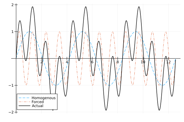
In this case the frequency of the forcing function is very different from the natural frequency of the system. This case is similar to the previous one, except that absent any damping neither the homogeneous and nor the particular solutions decay (they are both sinusoids with distinct frequencies). Thus the full solution will be the superposition or addition of two sinusoids.

Beats, i.e. $\omega \approx \omega_n$.

This is where $\omega \approx \omega_n$ and there’s no damping, so both the homogeneous and particular solutions are sinusoids. Moreover, the frequencies are close enough such that we have periodic cancellations between the homogeneous and particular solutions. An example solution of such a case is there in your homework. It is actually possible to show that when $\omega \approx \omega_n$, the solution will be a superposition of two sine waves with very similar frequencies leading to the presence of a high frequency component and a low frequency component in the solution. However,this requires a lot of algebra to show and isn’t going to significantly improve your life, so we don’t go into it here.

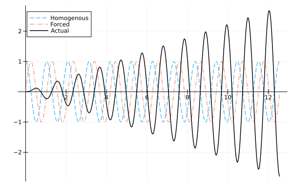
Resonance, i.e $\omega = \omega_n$.

This last case, as the title says is the case of resonance. Recall that for a inhomogeneous system:

the homogenous solution (i.e. obtained when $F(t) \equiv 0$) is given by: and we need to solve for the particular solution using the method of undetermined coefficients. But now $F(t) = \sin(\omega t)$ is a match for a homogenous basis function which results in a modification which means the particular solutions grow with time. Thus, in the case of resonance, the solution "blows up".

Electrical systems

We assume everyone is familiar with PHYS 212 material regarding basic electrical components like resistors, capacitors and inductors and Kirchoff's current (KCL) and voltage laws (KVL). In this section, we start by discussing how the differential equations arising from electrical circuits have analogues with the mechanical systems we were just discussing.

Analogues with mechanical systems

The basic relations to remember here from PHYS 212 are the equations for the voltage drops across the resistor, capacitor and inductor which are presented below in their most common form:

To start consider the basic RLC circuit shown below:

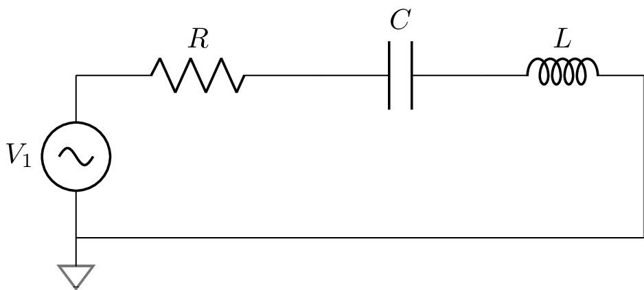
We can derive the differential equation governing this circuit via an application of KVL using the familiar rules above:

however if we switch the basic unit from current to charge $q$ such that $I=\dfrac{dq}{dt}$ then we can put the above equation in the form

$$L \ddot{q} = V_1 - R \dot{q} - \dfrac{q}{C}$$

which we say is analogous to the mass-spring-damper equation (1) because the variable substitutions $q \to x, V_1 \to F_{ext}, R \to c$ and $\dfrac{1}{C} \to k$ allow us to go between the two equations.

In fact we can derive more analogies based on these observations as summarized in the below table. The key points are:

• Capacitors store energy by accumulating charge akin to springs store energy under extension or compression. This accounts for potential energy.

• Inductors provide inertia against a change in the current flow through them and store energy via magnetic fields; thus providing an analogy with mass & energy associated with motion, i.e. kinetic energy.

• Dashpots/dampers and resistors both dissipate energy in a system by opposing motion, one via friction and the other via opposition to the motion of electrons.

Summary table

Type	Basic unit	Derivative	Storage	Energy	Dissipation	Driver	Inertia	Energy
Mechanical	Disp.[1]	Velocity	Spring	Potential	Friction	Force	Mass	Kinetic
Equations	$x$	$\dot x$	$k x$	$\dfrac{kx^2}{2}$	$c\dot x$	$F$	$M\ddot{x}$	$\dfrac{m\dot{x}^2}{2}$
Electrical	Charge	Current	Capacitor	Electric	Resistor	Voltage	Inductor	Magnetic
Equations	$q$	$\dot q$	$\dfrac{q}{C}$	$\dfrac{q^2}{2C}$	$R\dot q$	$V$	$L\ddot{q}$	$\dfrac{L\dot{q}^2}{2}$

Exercise: Find the mechanical analogue of the electrical system depicted below:

Impedance, a generalized resistance

We are familiar with the notion of calling the obstruction of the motion of electrons through a material as the characteristic resistance of a material. Naturally, conductors have very low resistance and insulators have extremely high resistance. Generally speaking, this applies to electrical circuit elements regardless of whether we are dealing with a DC (direct current) circuit or an AC circuit (alternating current) circuit. However, when it comes to inductors and capacitors, recall that their behavior is far more interesting in the AC case than in the DC case. Indeed, for example, with DC current, uncharged capacitors act like short circuits (transient phase) and fully charged capacitors (steady state) act like open circuits. Similarly, inductors in steady state can be considered short circuits and vice versa. It is precisely when the electric field changes continuously across the dielectric in a capacitor or within an inductor that our familiar equations

$$V = L\dfrac{dI}{dt} \qquad \textrm{and} \qquad I = C\dfrac{dV}{dt}$$

hold. It turns out that each of these circuit elements offer their own obstruction to the flow of AC, albeit in a frequency dependent manner. This obstruction term is called reactance.

In fact, (3) tells us even more. The first of these tells us that the voltage across the inductor is zero whenever the slope of the $I$ vs. $t$ (time) graph is horizontal and that $V$ is maximized when the rate of change of current is maximized. Thus if $I=sin(t)$ then $V$ is a cosine and vice versa. A similar relationship can also be seen to hold for the second equation above. This leads us to the following conclusions:

• Current lags voltage by $90^\circ$ in a purely inductive circuit

• Current leads voltage by $90^\circ$ in a purely capacitive circuit

Moreover, for an inductor, faster the current switches direction (consider AC) the larger the voltage drop and so is its contribution to the voltage drop in a circuit (i.e reactance) is directly proportional to the frequency $\omega$ of the applied AC. Conversely for a capacitor, faster the electric field switches, the more is the current. Thus its opposition to current (or reactance) is inversely proportional to the AC frequency. Thus we get the following definitions of inductive and capacitive reactance (denoted using a $X$):

Coupling this with inherent/internal Ohmic losses (i.e. pure resistance $R$) and the fact that the current/voltage relationship are out of phase with each other we defined the impedance for each of these elements as:

which dovetails nicely with our adopted notation for the Laplace domain variable $s = j \omega$ to give us the usual definition of impedances for the capacitor and inductor:

$$Z_L = L s \qquad \textrm{and} \qquad Z_C = \dfrac{1}{Cs}$$ Exercise: Make sense of the lead-lag relationship in the bullet points above for inductors/capacitors in conjunction with the definition of impedance in (4) and the generalized Ohm's law: $V=IZ$.

Solution: From the form of the generalized Ohm's law: $V=IZ$ the $Z$ term should appropriately add or subtract phase from the current to give the right relationship with velocity. Considering the Argand plane

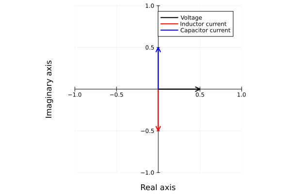
we see that $Z_L$ should add a phase of $\pi/2$ whereas $Z_C$ subtracts a phase of $\pi/2$. This meshes well with the bullet points above since:

• For inductors we take the lagging current and add $\pi/2$ to get voltage with the correct phase.

• For capacitors we take the leading current and subtract $\pi/2$ to get voltage with the correct phase.

This is another example where algebra and math is simplified using "imaginary" numbers.

[back]

[1]	Displacement: Just trying to make the table fit. 😁