Lecture 14

Reading material: Chapter 7 and 9 of CSSB

In the last lecture we talked about using the Laplace transform to solve convolutions, ODEs, and IVPs and along the way we encountered partial fraction expansions. In this lecture we take a detailed look at second order systems and associated theory along with an applet/demonstration. Finally we will also start our introduction to Simulink.

Second order systems
Simulink

Second order systems

Recall that the prototypical second order system is represented by the transfer function:

\begin{aligned} H(s) &= \frac{\omega^2_n}{s^2 + 2\zeta\omega_n s + \omega^2_n}, \end{aligned}

where

$\zeta$ is a non-negative and $\omega_n$ is strictly positive and are called the damping ration and natural frequency respectively;
the denominator is a general second degree monic polynomial;
$H(s)$ is normalized so that $H(s=0)=1$ .

By the quadratic formula we get that the denominator has roots (called poles):

s = - \zeta \omega_n \pm \omega_n \sqrt{\zeta^2 - 1}

Therefore the nature of the poles depend on $\zeta$ .

if $\zeta >1$ , both poles are real and negative - called overdamped
if $\zeta=1$ then there are two repeated real negative poles - called critically damped
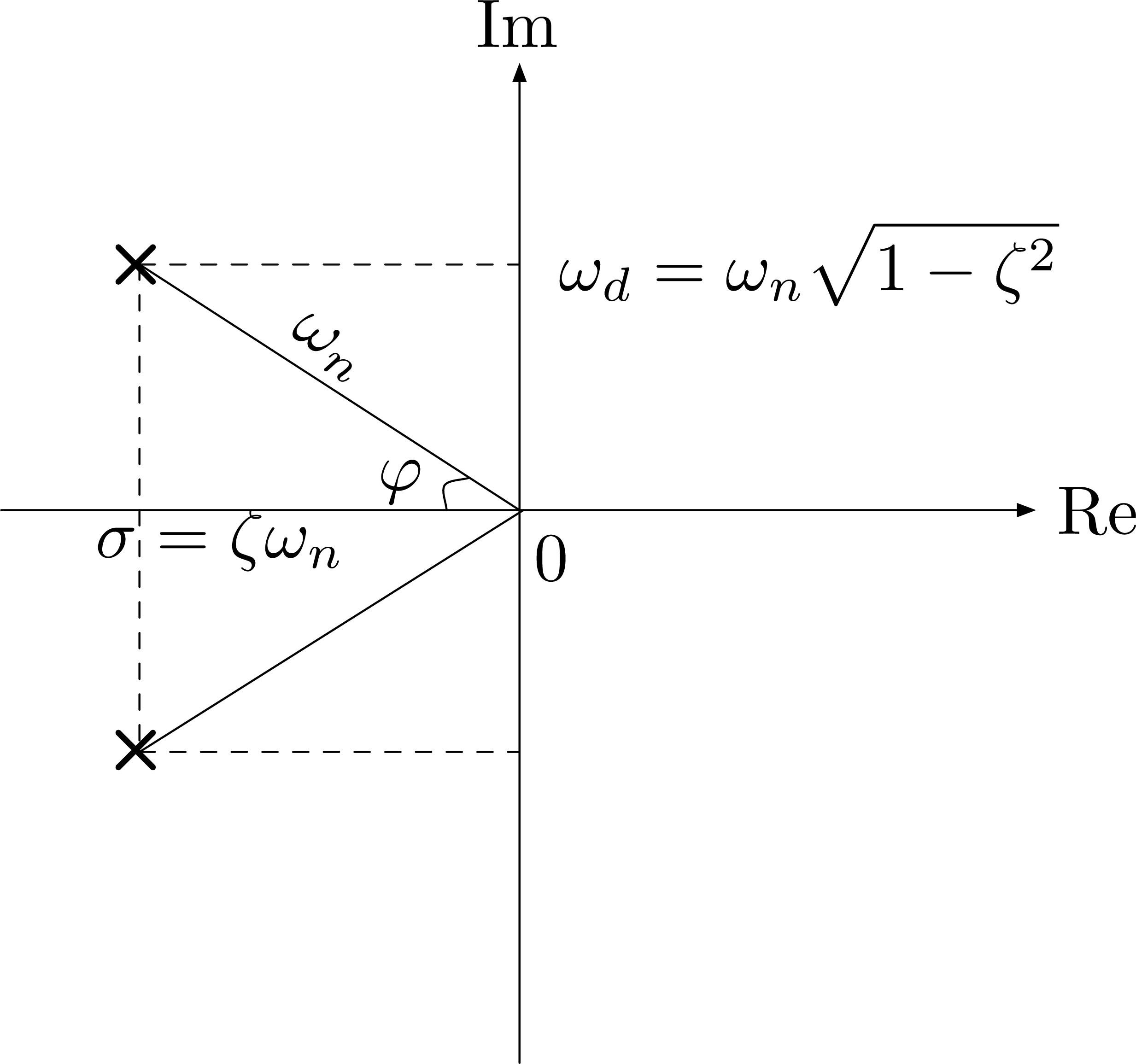
if $\zeta <1$ then there are two complex poles with negative real parts $s = - \sigma \pm j \omega_d$ where $\sigma = \zeta \omega_n$ and $\omega_d = \omega_n \sqrt{1 - \zeta^2}$ - called the underdamped case

Let us consider the underdamped case. For the underdamped system the roots are:

\begin{aligned} s &= -\zeta \omega_n \pm j \omega_n \sqrt{1 - \zeta^2} \\ &= -\sigma \pm j \omega_d \end{aligned}

we can plot the complex valued poles in the complex plane as follows:

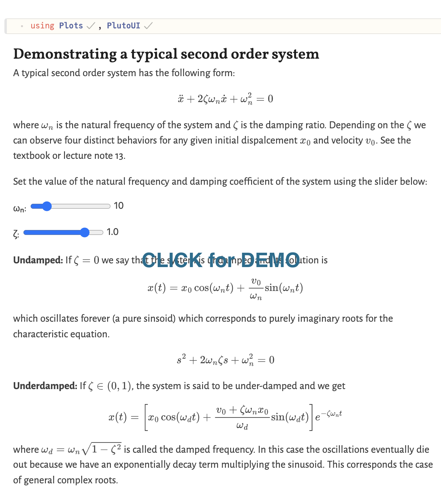
If we compute the time domain system response to an impulse we get:

\begin{aligned} h(t) &= \mathcal{L}^{-1}\{ H(s)\} \qquad \qquad \qquad \quad \textrm{(by definition of transfer function)}\\ &= \mathcal{L}^{-1}\left\{ \frac{\omega^2_n}{s^2 + 2\zeta\omega_n s + \omega^2_n} \right\}\\ &= \mathcal{L}^{-1}\left\{ \frac{\omega^2_n}{(s+\sigma)^2 + \omega^2_d} \right\} \qquad \textrm{(by the above underdamped poles)} \\ &= \mathcal{L}^{-1}\left\{ \frac{(\omega^2_n/\omega_d)\omega_d}{(s+\sigma)^2 + \omega^2_d} \right\} \\ &= \frac{\omega^2_n}{\omega_d}e^{-\sigma t}\sin(\omega_d t) \quad \qquad \qquad \textrm{(by transform tables)} \end{aligned}

and that to a step response as:

\begin{aligned} y(t) &= \mathcal{L}^{-1}\left\{ Y(s) \right\} \\ &= \mathcal{L}^{-1}\left\{ \frac{H(s)}{s} \right\} \\ &= \mathcal{L}^{-1}\left\{ \frac{\sigma^2 + \omega^2_d}{s[(s+\sigma)^2 + \omega^2_d]} \right\} \qquad \qquad \qquad \textrm{(from plot above)}\\ &=1-e^{-\sigma t} \left(\cos(\omega_d t) + \frac{\sigma}{\omega_d}\sin(\omega_d t)\right) \qquad \textrm{(by transform tables)} \end{aligned}

The demonstration below (click to go there) allows you to visualize the system response for different values of $\zeta$ . From here we see that, the decaying rate of the exponential in step response depends on the real part of the pair of complex poles, i.e. $-\sigma = - \zeta \omega_n$ whereas the imaginary part determines how the step response oscillates while it decays. This is the reason for calling $\omega_d = \omega_n \sqrt{1 - \zeta^2}$ the damped natural frequency. The other cases are also discussed in detail in the demonstration.

Simulink

Simulink will be covered in Class. See Homework 10 and also see the activity below.

Some other useful links are:

Simulink Onramp which is part of homework.
A tutorial from Michigan.
A dated tutorial from Nevada
A less dated one from Florida

[back]

CC BY-SA 4.0 Ivan Abraham. Last modified: April 30, 2023. Website built with Franklin.jl and the Julia programming language. Curious? See familiar examples.