Lecture 10

Reading material: Chapter 5 of CSSB

In the last lecture we wrapped up the first part of CSSB^[1] and from this lecture note onwards we are in the second part which is all about analysis of systems. We start by laying the groundwork with concepts of impulse response, frequency response and convolutions which help completely characterize single input, single output (SISO) linear time invariant (LTI) systems.

Consequences of linearity
The impulse function
Impulse & convolution in the frequency domain
Digital implementation
1. Code examples
2. Filtering using convolution

Consequences of linearity

Recall that we loosely described linearity as the characteristic of a system that shows "proportionality in response". More formally a system that is linear satisfies the additivity and homogeneity properties.

The latter means that if the input is scaled by some factor then so is the output. That is, if $f$ is a system that takes a (possibly vector) input $x$ and outputs $f(x)$ then $f( \alpha x) = \alpha f(x)$ for all scalars $\alpha$ . The additivity property means that when provided an input that is the addition of two quantities, the system output can be described as the sum of the outputs to the individual quantities, i.e. $f(x_1 + x_2) = f(x_1) + f(x_2)$ . Together, these properties are said to endow linear systems with the superposition principle.

Thus, for linear systems and in particular linear time-invariant systems (LTI), to understand the system's response to very complicated inputs, it suffices to break apart the input into small manageable pieces, calculate its response to these pieces, and then sum it all up together and this is precisely what impulse functions let us do.

The impulse function

We are already familiar with the definition of the impulse function as the idealized signal $\delta(t)$ which is only nonzero at time $t=0$ and takes on an amplitude such that

\int _{\mathbb{R}} \delta (x) dx = 1

One important property of the impulse function is called the sifting property which is best explained as follows. Consider

\int_{\mathbb{R}} f(s) \delta (s - t) ds = \int_{\mathbb{R}} f(t) \delta(s - t) ds = f(t) \int _{\mathbb{R}} \delta(t-s) ds = f(t)

where we have used the fact that the impulse $\delta(s-t)$ is only nonzero when $s=t$ to change $f(s)$ to $f(t)$ . Then we pull it out of the integral because it doesn't depend on the integration variable. At the final step we use the unit area property to calculate the integral as 1. Thus ,we see that the impulse function has the ability to pick out a single value amongst all the values $f(t)$ could take.

Now, we are quite familiar with the notion of changing to the frequency domain via the Fourier transform as a change of basis to complex exponentials or equivalently to sinusoid. Then, let us take a step back and ask the following question.

Recall that in the case of the continuous Fourier transform, we had

f(t) = \dfrac{1}{\sqrt{2 \pi}} \int \limits _{-\infty} ^{\infty} F(\omega) e^{i \omega t } d\omega

with the interpretation being that we are synthesizing

f(t)

by integrating over all possible frequencies

\omega

, continuously weighted by the function

F(\omega)

. Then, by using the impulse function

\delta (t)

we could also write:

f(t) = \int \limits _{-\infty} ^{\infty} f(s) \delta (s-t) ds \qquad \forall t \in \mathbb{R}

We can interpret the above as an expression of $f(t)$ in terms of continuum of "basis" functions given by $\delta(s-t)$ for each value of $t$ .

As we remarked, by the principle of superposition, for linear systems it suffices to figure out what the system's response is to individual inputs. Since we can represent $f(t)$ in the time domain as a continuously weighted sum/integral of the impulse function, it turns out that the response of LTI systems to the impulse function (called the impulse response) characterizes its response to any and all inputs.

Recall that for time invariant systems, time shifting the input $x(t)$ is the same as time shifting the output $y(t)$ , i.e.: $y(t-T) = f(x(t-T))$ . Therefore the above is a powerful statement that tells us we can find the response of an LTI system to arbitrarily complex inputs by simply weighting and summing (or integrating) its responses to a sequence of shifted impulses.

An LTI system is completely characterized by its response to the impulse function.

Convolution

The operation performed in (1) is common enough in signal processing to warrant its own name: convolution. Some sources denote convolution with a $\ast$ but this is often confusing because of the wide use of $\ast$ to denote multiplication, especially on computers. Therefore we will use $\star$ instead.

Definition: (Convolution) The convolution of two functions $f$ and $g$ is defined as

f(t) \star g(t) = \int \limits _{-\infty} ^{\infty} f (\tau) g (t - \tau) d \tau

Using convolution we can represent the output of any LTI system to an input $x(t)$ using its impulse response $h(t)$ as:

y(t) = x(t) \star h(t) = \int \limits_{-\infty} ^{\infty} x (t - \tau) \cdot h(\tau) d\tau = \int \limits_{-\infty} ^{\infty} x (\tau) \cdot h(t-\tau) d\tau

where we have used the fact that convolution operation is commutative to get the second equality.

Possible homework problem.

The astute reader may have noticed the similarity of (2) with that of the definition of the cross correlation of two functions. Indeed one can think of convolution of $f(t)$ with $g(t)$ as the cross-correlation of $f(t)$ with $g(-t)$ or $f(-t)$ with $g(t)$ . Thus the main difference is that in convolution, one of the signals is reversed in the time axis. For calculating the system response, CSSB explains this reversal as:

When implementing convolution, we reverse the input signal, because it is the input signal’s smallest time value that produces the initial output.

but you might as well accept it as a definition. To see visually the difference between convolution and cross-correlation, see below image from Wikipedia:

⚠️ Note

It is imperative to understand intuitively what convolution of two signals in the time domain looks like graphically. See this excellent demonstration.

Example

Let us find the convolution of $f(t) = e^{-t}$ and $g(t)=\sin(t)$ over the non-negative real line. By definition we have that

\begin{aligned} f(t) \star g(t) &= \int \limits _{0} ^{t} e^{-\tau} \sin (t- \tau) d \tau \\ &= \left[ e^{-\tau} \cos(t-\tau) \right] _{0}^{t} - \left[ e^{-\tau} \sin (t - \tau) \right]_0^{\tau} - \int \limits _0 ^t e^{-\tau} \sin (t - \tau ) d\tau \end{aligned}

Rearranging we have,

\begin{aligned} 2 \left( f(t) \star g(t) \right) &= \left[ e^{-\tau} \cos(t-\tau) \right] _{0}^{t} - \left[ e^{-\tau} \sin (t - \tau) \right]_0^{\tau} \\ & = e^{-t} - \cos(t) - 0 + \sin(t) \\ \implies f(t) \star g(t) &= \dfrac{1}{2} \left ( e^{-t} + \sin(t) - \cos(t) \right) \end{aligned}

⚠️ Note

Discrete time: For an example in discrete time, check Example 5.4 in CSSB in detail.

Visual example(s)

The animation below shows the result of convolving two square pulses.

Impulse & convolution in the frequency domain

The impulse function is intimately related to Fourier transform because of the simple fact that the Fourier transform of the unit impulse function is unity. Indeed we have that,

\mathcal{F}_{\delta}(\omega) = \int \limits _{-\infty} ^{\infty} \delta (t) e^{-i \omega t} dt = \int \limits _{-\infty} ^{\infty} 1 \cdot e^{-i\omega t} dt = \left. e^{-i\omega t}\right|_{t=0} = 1

This is an important property of the impulse function because it allows us to characterize the so called spectrum of the system. In other words, since the impulse function has a constant amplitude across all frequencies, the system response to the impulse response tells us exactly what it does to signals at each frequency.

Left as an exercise.

By considering the above properties we can show the below Fourier transform pairs:

Time domain	Frequency domain
$\delta(t)$	$1$
$1$	$2\pi \delta (\omega)$
$\cos(\omega_0t)$	$\pi \left( \delta( \omega + \omega_0 ) + \delta ( \omega - \omega_0) \right)$
$\sin(\omega_0t)$	$i \pi \left( \delta( \omega + \omega_0 ) + \delta ( \omega - \omega_0) \right)$

Now let us turn our attention to the question of what is the equivalent of the convolution operator in the frequency domain. After all, we started this course proclaiming that the time and frequency domain representations of signals are equivalent. Therefore, it is only practical that we examine what happens to the all important convolution operation used to define the time response of LTI systems via the impulse response in the frequency domain. Let us take the Fourier transform of the convolution of two functions:

\begin{aligned} \mathcal{F} \left( f(t) \star g(t) \right) &= \mathcal{F} \left( \int \limits _{-\infty} ^{\infty} f(\tau) g(t-\tau) d \tau \right) \\ & = \int \limits _{-\infty} ^{\infty} \int \limits _{-\infty} ^{\infty} f(\tau) g(t-\tau) d \tau \cdot e^{-i\omega t} dt \\ & = \int \limits _{-\infty} ^{\infty} f(\tau) \int \limits _{-\infty} ^{\infty} g(t-\tau) e^{-i\omega t} dt \cdot d \tau \\ & = \int \limits _{-\infty} ^{\infty} f(\tau) G(\omega) e^{-i\omega \tau} d\tau = G(\omega) \int \limits _{-\infty} ^{\infty} f(\tau) e^{-i\omega \tau} d\tau \\ & = G(\omega) F(\omega) \end{aligned}

where in the third line we changed the order of integration and in the following line we used the fact that the Fourier transform of a time shifted version of a function is its Fourier transform multiplied by an exponential determined by the shift. In other words, if $X(\omega)$ is the Fourier transform of $x(t)$ then $\mathcal{F} ( x(t- \tau) )$ is $X(\omega) \cdot e^{-i\omega \tau}$ .

Exercise: Prove the above property about time shifts.

Thus we see that convolution in the time domain becomes multiplication in the Fourier domain. The reverse also holds true, namely convolution in the frequency domain becomes multiplication in the time domain. This observation accords us a strategy to avoid performing convolution and stick with multiplication, to find the system response, that is, if we are willing to tolerate an inverse Fourier transform. The strategy is as follows:

Take the Fourier transform of the impulse response $h(t)$ and the input to the system $x(t)$ to get $H(\omega)$ and $X(\omega)$ respectively.
Perform the multiplication in the frequency domain: $Y(\omega) = H(\omega)X(\omega)$ .
Take the inverse Fourier transform $y(t) = \mathcal{F}^{-1} \left(Y (\omega) \right)$ .

Now that we have established the relationship between the time and frequency domains for the impulse function, now is a good time to review properties of the Fourier transform.

Some properties of the Fourier transform.

We state the following properties in the below table without proof.

Name	Time Domain	Frequency Domain
Linearity	$\alpha x_1(t) + \beta x_2(t)$	$\alpha X_1(\omega) + \beta X_2 (\omega)$
Time scaling	$x(t/a)$	$aX(\omega a)$
Time delay	$f(t-a)$	$X(\omega) e^{-i\omega a}$
Complex shift	$x(t)e^{i\omega_0 t}$	$X(\omega - \omega_0)$
Time reversal	$f(-t)$	$F(-\omega)$
Convolution	$x(t) \star h(t)$	$X(\omega)H(\omega)$
Multiplication	$x(t)y(t)$	$X(\omega) \star Y(\omega)$
Differentiation	$\dfrac{d^n x(t)}{dt^n}$	$(i\omega)^n X(\omega)$
Time multiplication	$t^n x(t)$	$i^n \dfrac{d^n}{d\omega^n} X(\omega)$

Digital implementation

By now we know that almost always, on a computer, functions and signals are all represented by a list of numbers. Therefore, the discrete version of the convolution is what gets really implemented:

\left(f \star g \right) [n] = \sum \limits _{m = - \infty} ^{\infty} f[m]g[n-m]

Here is a visual example of what that looks like:

As usual, people far smarter than me have worked on making these somewhat mathematical topics accessible to everyone. In particular, Grant Sanderson has produced an excellent video on the topic of convolution, that I would highly recommend watching. Moreover, the interested student should definitely, check out a few other videos that he references (e.g. regarding the DFT algorithm).

Hopefully, having developed some more intuition about convolution, now let us turn to the issue of the impulse function in the digital domain.

Impulse function

Of course the impulse function is an idealization - in fact it is not even a real function in the mathematical sense, rather we have defined it via the properties it should have. But this leaves open the question of how to implement something so idealized on a digital machine. The approach we take is to ask: "What is a good enough approximation to the impulse function?

The answer, as is often in life, is it depends. In particular, it depends on the signal/system characteristics that we are analyzing. In the below figure we plot the magnitude spectrum for a few pulse signals on the left. The pulses are 1 ms, 2 ms and 5 ms long each and the DFT assumes a sampling frequency of 1 kHz. We see that only the true discrete impulse function (1 for the first sample and zero after) has the expected characteristic.

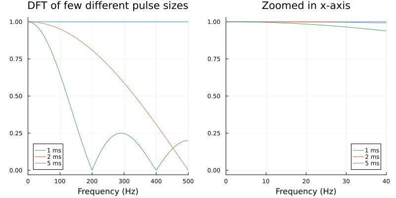
Now consider a system whose characteristic is akin to a low pass filter with a cutoff of 2 Hz. If we zoom-in on the $x$ -axis we see that even the 2 ms pulse can serve as an impulse function over this frequency range.

Convolution

In MATLAB there are two functions that implement convolution. There are the conv and filter functions with the latter being a far more general function. For the former, the function signature is as follows:

y = conv(x, h, 'shape')

where x and h are the input signals and shape is a parameter that specifies what the output should look like.

Parameter	Output length	Function
`full`	$l_x +l_h -1$	Zero pads as necessary
`same`	$l_x$	Zero pads but only returns central sum
`valid`	$l_x -l_h -1$	No zero padding

Note that in either cases the output will require normalization by the length of samples.

Code examples

Consider the following MATLAB code:

x=1:6
y=1:5

default = conv(x, y)
default_flip = conv(y, x)

valid = conv(x, y, 'valid')
valid_flip = conv(x, y, 'valid')

same = conv(x, y, 'same')
same_flip = conv(y, x, 'same')

and carefully observe the output:

default =
     1     4    10    20    35    50    58    58    49    30

default_flip =
     1     4    10    20    35    50    58    58    49    30

valid =
    35    50

valid_flip =
    35    50

same =
    10    20    35    50    58    58

same_flip =
    20    35    50    58    58

As you can see, only the full (default) mode of convolution preserves its commutativity. The equivalent of conv(h, x) using the filter command in MATLAB is filter(h, 1, x).

Convolution/multiplication relation

We remarked that convolution in the time domain is equivalent to multiplication in the frequency domain. This below example, based on CSSB Example 5.7 shows that this is indeed the case. Clicking on the image will get you the code that generated it for the website, and in Chapter 5 you can find the Python code.

The equivalent MATLAB code from CSSB is shown below for completeness sake.

% Example 5.7  Given the system impulse response below, find the output of the system
%    to a sawtooth wave (Figure 5.20)having a frequency of 400 Hz.
%   Use both convolution and frequency domain approaches.
%   Also find an plot on a dB-semilog scale the transfer function of the system.
%  Since the sawtooth has a frequency of 3.2 Hz, we will use a sampling interval of 4 kHz
%
close all; clear all;
fs = 160;                       % Sample frequency
T = 1;                          % Time in sec;
t = (0:1/fs:T);                 % Time vector
N = length(t);                  % Determine length of time vector
x = sawtooth(20*t-pi/2,.5);              % Construct input wave
h = 5* exp(-5*t).*sin(100*t);
subplot(1,2,1)
plot(t,x,'k');
title('A) Input Signal','FontSize',12);
xlabel('Time (sec)','FontSize',14);  ylabel('x(t)','FontSize',14);
ylim([-1.2 1.2]);
subplot(1,2,2);
plot(t,h,'k');
title('B) Impulse Response','FontSize',12);
xlabel('Time (sec)','FontSize',14);  ylabel('h(t)','FontSize',14);
% Calculate output using convolution.
y = conv(x,h);             % Calculate output
figure;
subplot(2,1,1)
    plot(t,y(1:N),'k'); hold on;
    title('Time Domain (convolution)','FontSize',12);
xlabel('Time (sec)','FontSize',14);  ylabel('y(t)','FontSize',14);
% Now calculate in the frequency domain.
TF = fft(h);            % Take Fourier transform of iimpulse response
X = fft(x);             % Take Fourier transform of input
Y = X.*TF;              % Take product in the frequency domain
y1 = ifft(Y);           % Take the inverse fourier transform to get y(t)
subplot(2,1,2)
plot(t,y1,'k');
title('Freqeuncy Domain (multiplication)','FontSize',12);
xlabel('Time (sec)','FontSize',14);  ylabel('y(t)','FontSize',14);

⚠️ Note

With regards to implementation, remember that everything on a computer is done using DFT and that the DFT assumes periodicity of the input sequences. Therefore, on a computer the equivalence or relation between convolution in the time domain and multiplication in the Fourier domain holds proper for circular convolution. To see this in action, simply try adding a time shift of

\pi/2

to the sawtooth wave in the above code and look at the output. To know more about this very common source of error: go here.

Filtering using convolution

Considering our discussion of digital or discrete convolution above, it is straightforward to note that whenever one of the sequences $f[n]$ or $g[m]$ is a constant, we end up performing some sort of weighted averaging. In particular, when the constants are $\dfrac{1}{n}$ or $\dfrac{1}{m}$ we get an $n$ or $m$ point moving average if the sequences $f$ and $g$ are also of length $n$ or $m$ respectively as shown in below figure (you are encouraged to write down the MATLAB version of the code).

N, t = 10, 0:0.01:2π 		# We are taking N=10 point average  
f(t) = sin(t) + rand()		# Generates a noisy sinusoid
plot(t, f.(t), label="Noisy sine") 	# Plots it
z(t) = conv(f.(t), repeat([1/N],N))	# Convolve with a constant vector

# Convolution result may be different length than time vector 
# but result is still on [0, 2π]

plot!(LinRange(0, 2π, length(z(t))), z(t), label="Smoothened sine", 
	title="Taking 10 point average")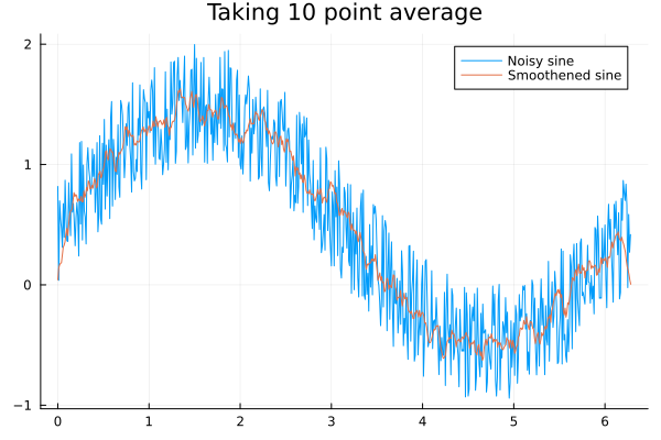

[back]

[1]	CSSB is divided into three parts, signals, systems and circuits.

CC BY-SA 4.0 Ivan Abraham. Last modified: March 22, 2023. Website built with Franklin.jl and the Julia programming language. Curious? See familiar examples.