Lecture 09

Reading material: Chapter 4 of CSSB

Last time we discussed implementing different reconstructions of signals based on their Fourier coefficients in a programming language. We also discussed the use of the FFTW library to perform the Fast Fourier Transform in MATLAB or some other programming language. Further, in class we did an example where we took the Fourier transform of a sound wave. The notes/notebook we used in class is accessible here.

⚠️ Note

If you haven't understood how to take the Fourier transform of a signal using MATLAB or some other software, then stop here. Read the previous lectures, check out the above notebook and catch up before proceeding.

Sampling
1. The sampling rate & constraints
2. Sampling theorem
Power spectral density
Spectrograms & windowing
Spectral leakage
1. Bandwidth
Conclusion

Sampling

In this lecture we want to study the effect of sampling on the DFT spectrum. The vast majority of real life signals are continuous time signals. However, our primary methods of analyzing them are all based on computers. Thus there arises a central question: When is a sampled signal a good^[1] representation of its continuous time counterpart?

We start, as you must have guessed, but looking at sinusoids.

The sampling rate & constraints

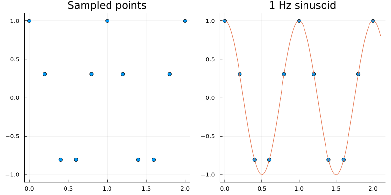
Consider the left plot above which we can suppose we got by sampling some signal. Intuitively, we might guess that we must have sampled some sort of periodic waveform like a sinusoid. And indeed as shown on the right we see that a 1 Hz. cosine neatly fits through those points. However, is this the only signal that could have generated those sampled points?

Indeed, consider the plots below.

Therefore it is possible to get the same sampled sequence of points from different signals; and this phenomenon is called aliasing.

Definition: (Aliases) Given a sampling frequency

f_s

, two frequencies

f_1

and

f_2

are called aliases of each other if for some integer

k

f_2 = f_1 + k\cdot f_s

One of the primary concerns when dealing with sampled signals is to avoid aliasing because then we will not be able to tell apart signals of different frequencies. Fortunately for us, this problem has been solved by folks at Bell Labs in its heyday but before we get to that, here is another question:

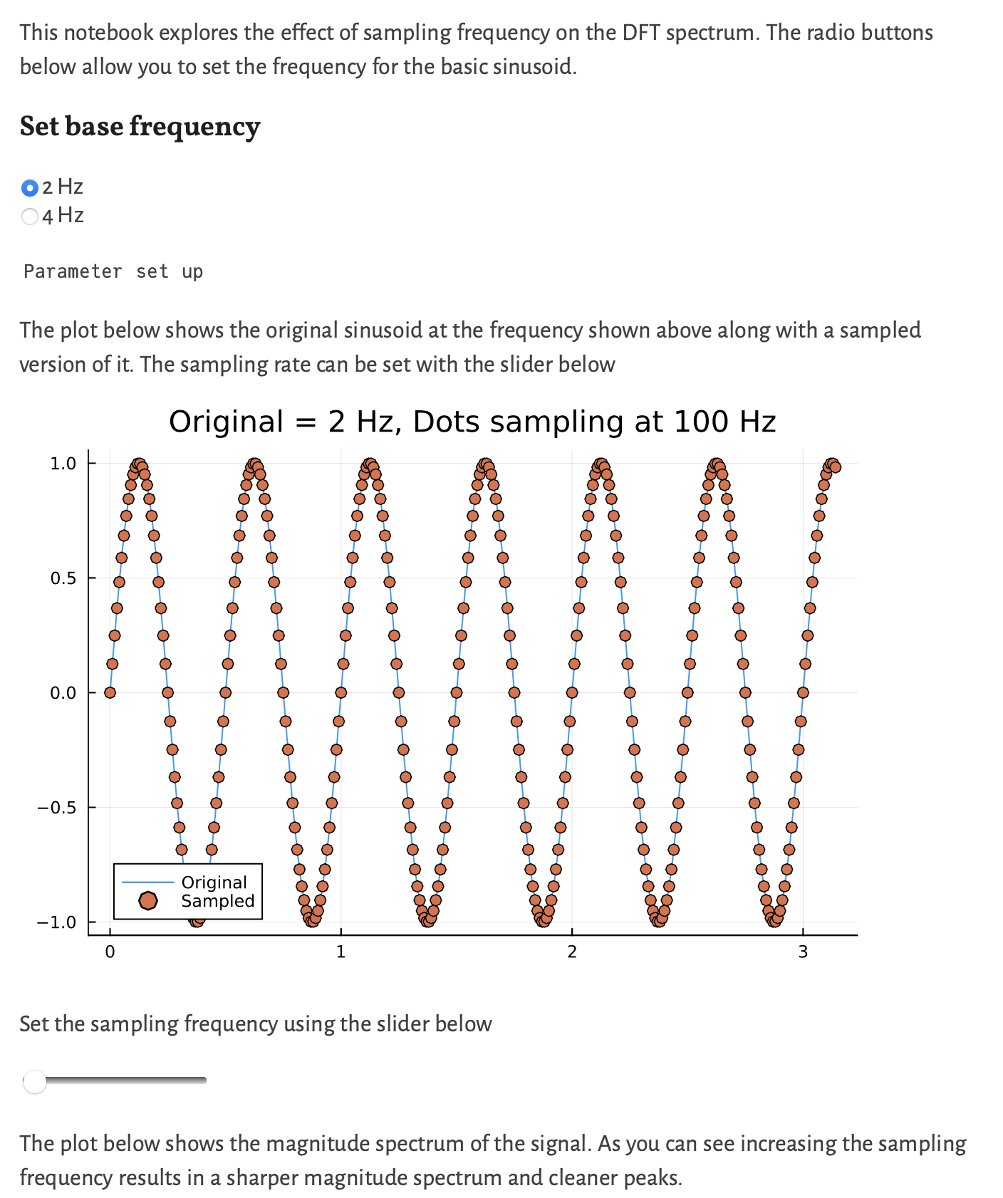
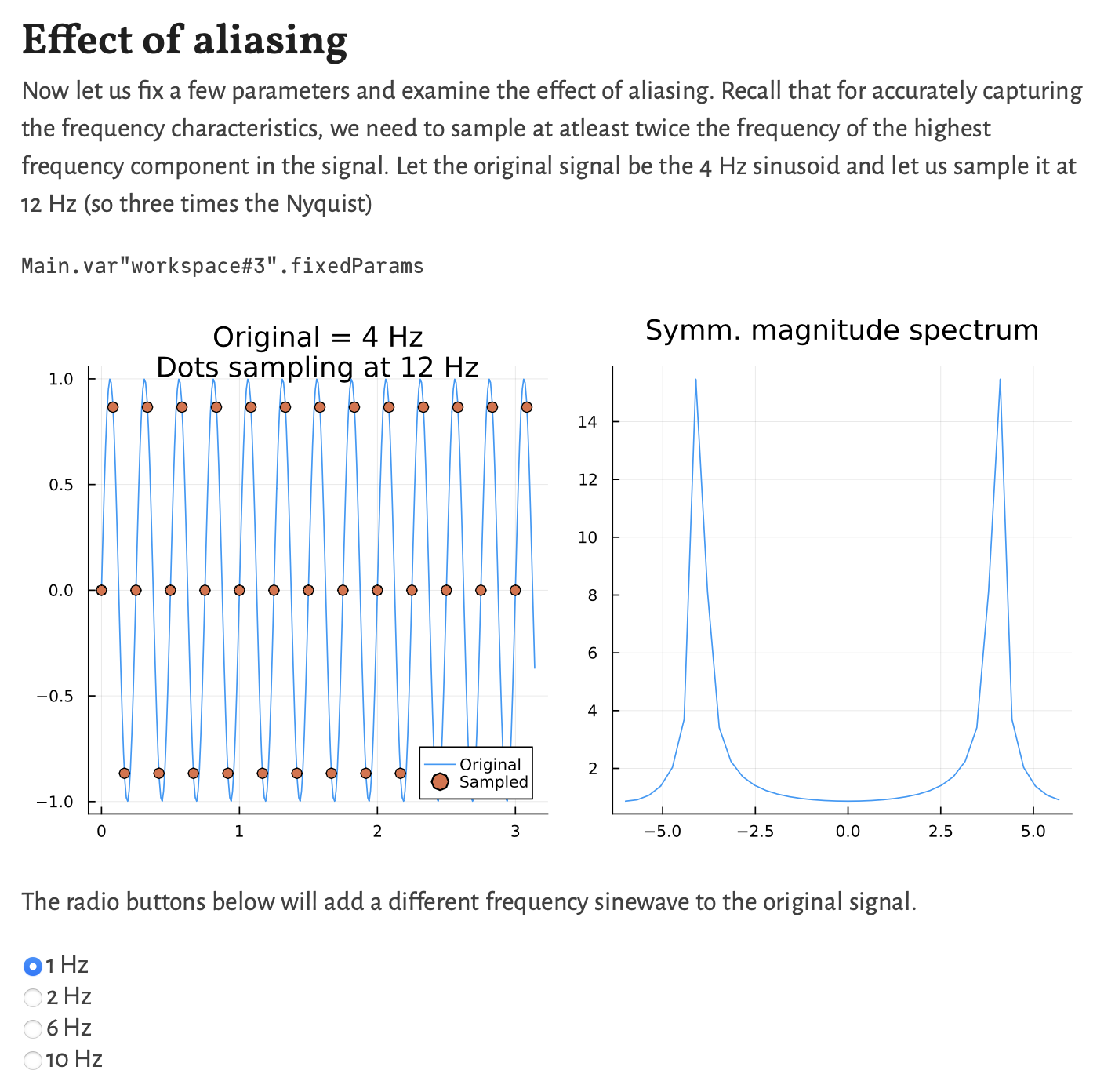
What is the effect of the sampling rate on the DFT spectrum?

The demonstration below allows you to explore this question:

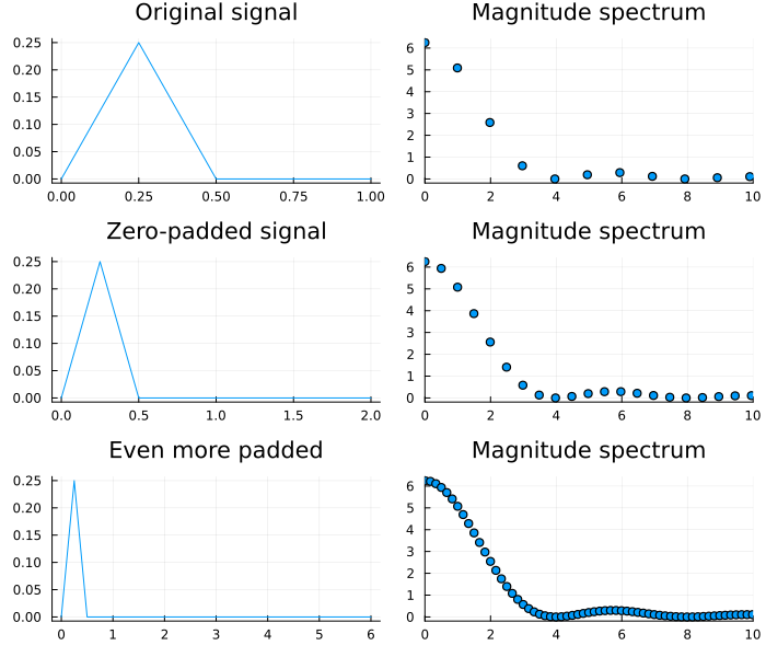
In the above we saw that increasing the number of samples that is passed to fft allows us to get sharper peaks with greater resolution. Thus zero padding is a frequent technique used by people to "increase" the resolution of a DFT magnitude spectrum. Of course zero padding doesn't add any new information, so it really amounts to an aesthetic trick, albeit with some consequences^[2] but more on that later. The plot below shows the DFT of the same signal without zero padding, with some zero padding, and with even more zero padding.

Sampling theorem

So now that we have seen what effect the length of the input sample, or rather the sampling rate has on the DFT spectrum, let us return to the original problem involving sampling. The central result here is called Shannon's Sampling Theorem after the great polymath Claude Shannon though it often (and rightly) has various other names associated with it.

Theorem: (Shannon) If a signal

y(t)

contains no frequencies higher than

f

hertz, it is completely determined by sampling its values at a series of points spaced

1/(2f)

seconds apart.

We have already seen this result and remarked upon it in class. Indeed in the above demonstration, one can check that for a $4$ Hz wave, setting the sampling frequency to $8$ Hz (via the slider) results in a flat line. The same effect can also seen in the DFT magnitude spectrum.

Power spectral density

As we have seen in a previous demonstration using a sound file, the phase spectrum returned by the DFT can be unhelpful or hard to interpret. Instead in signal processing we often prefer to look at how much of the signals power is concentrated in its different frequency components. This is done by looking at its power spectral density (PSD) plot. Recall that power is defined as the rate of change of energy. Similar to how we compute the distance covered from a velocity time graph (by integration), we can compute the total energy content in a signal as

E_ x = \int \limits _{-\infty} ^{\infty} |x(t)| ^2 dt

On the other hand, the frequency and time domain representations of a signal are equivalent and therefore it should be possible to compute the energy in the frequency domain as well. The Parseval - Plancherel theorem provides us with exactly this equality.

\int \limits _{-\infty} ^{\infty} |x(t)|^2 dt = \int \limits _{-\infty} ^{\infty} |X(\omega)|^2 d\omega = \int \limits _{-\infty} ^{\infty} X(\omega) \cdot \overline{X(\omega)} d\omega

Where we got theh second equality using the properties of complex numbers. A little bit of manipulation then bring us to the traditional definition of the PSD as the Fourier transform of the signals autocorrelation function.

\begin{aligned} \int \limits _{-\infty} ^{\infty} X(\omega) \cdot \overline{X(\omega)} d\omega &= \int \limits _{-\infty} ^{\infty} \left[ \int \limits _{-\infty} ^{\infty} x(t) e^{-i \omega t} dt \cdot \int \limits _{-\infty} ^{\infty} x(s) e^{i \omega s} ds \right] d \omega \\ &= \int \limits _{-\infty} ^{\infty} \left[ \int \limits _{-\infty} ^{\infty} \int \limits _{-\infty} ^{\infty} x(t) x(s) e^{-i\omega(t-s)} dt \cdot ds \right] d\omega\\ &=\int \limits _{-\infty} ^{\infty} \left[ \int \limits _{-\infty} ^{\infty} \int \limits _{-\infty} ^{\infty} x(s+\tau) x(s) ds \cdot e^{-i\omega \tau } d\tau \right] d\omega \\ &=\int \limits _{-\infty} ^{\infty} \int \limits _{-\infty} ^{\infty} r_{xx}(\tau) \cdot e^{-i\omega \tau } d\tau \cdot d\omega = \int \limits _{-\infty} ^{\infty} \mathcal{F}_{r_{xx}}(\omega) \cdot d\omega \end{aligned}

Definition: (Power spectral density) Given a signal $x(t)$ its power spectral density is defined

\operatorname{PSD}_x(\omega) = \lim \limits _{T \to \infty} \dfrac{1}{T}. \int \limits _{-T/2} ^{T/2} r_{xx}(\tau) e^{-i\omega \tau} d\tau

The above, while being the classical definition is rarely used in practice. Instead one prefers to directly compute it from the magnitude of the DFT vector (from (1)). The animation below shows the normalized power spectral density remaining essentially constant while the sampling rate is being changed.

In MATLAB the functions periodogram and pwelch can be used to construct PSD plots. The difference between the two is that Welch's method uses localized averaging to reduce noise. While these routines are part of the expensive Signal Processing Toolbox, CSSB provides the following equivalent for our purposes.

function [PS,f] = welch(x,nfft,noverlap,fs)
%Function to calculate averaged spectrum
%[ps,f] = welch(x,nfft,noverlap,fs);
%  Output arguments
%		sp	spectrogram
%		f	frequency vector for plotting
%  Input arguments
%		x data
%		nfft window size
%      	noverlap number of overlaping points in adjacent segements
%	    fs sample frequency
%	Uses Hanning window
%
N = length(x);                     % Get data length
half_segment = round(nfft/2);      % Half segment length
if nargin < 4                      % Test inputs
    fs = 2*pi;                     % Default fs
end
if nargin < 3 || isempty(noverlap) == 1
    noverlap = half_segment;       % Set default overlap at 50%
end
nfft = round(nfft);                % Make sure nfft is an interger
noverlap = round(noverlap);        % Make sure noverlap is an interger
%
f = (1:half_segment)* fs/(nfft);   % Calculate frequency vector
increment = nfft - noverlap;       % Caluclate window shift
nu_avgs =  round(N/increment);     % Determine the number of segments
%
for k = 1:nu_avgs 			       % Calculate spectra for each data point
   first_point = 1 + (k - 1) * increment;
   if (first_point + nfft -1) > N
       first_point = N - nfft + 1;          % Prevent overflow
   end
    data = x(first_point:first_point+nfft-1); % Get data segment
    if k == 1
       PS = abs((fft(data)).^2);            % Calculate Power spectrum Eq. 4.16
   else
       PS = PS + abs((fft(data)).^2);       % Calculate Power spectrum
   end
end
PS = PS(2:half_segment+1)/(nu_avgs*nfft/2);  % Remove redundant points, no avg
end

Spectrograms & windowing

For signals that change their characteristics significantly over a period of time, the Fourier transform of the entire signal is often not all that informative. For example consider the below plot of data from a vibration sensor (data available from this website) along with a plot of its magnitude spectrum.

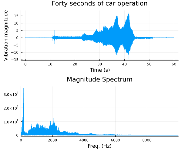
By looking at the time domain signal it is clear that there were four distinct modes of operation during the period of observation. The first ten seconds or so are flat, then the car is on and idling, before it is revved for a bit beginning at around 25 seconds. Finally it is left to idle again for a while before being turned off. None of this detail is visible in the frequency domain.

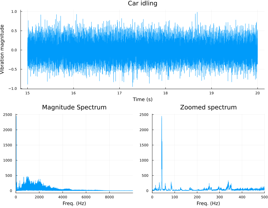
On the other hand, consider the below plot where the DFT was taken only for a portion of the signal when the car was found to be idling. The overall magnitude spectrum definitely shows a change.

One method of displaying partial time domain information along with the frequency spectrum is to construct spectrograms. This is done by chopping up the time domain signal into small overlapping segments. These FFT of these segments is then stitched together.

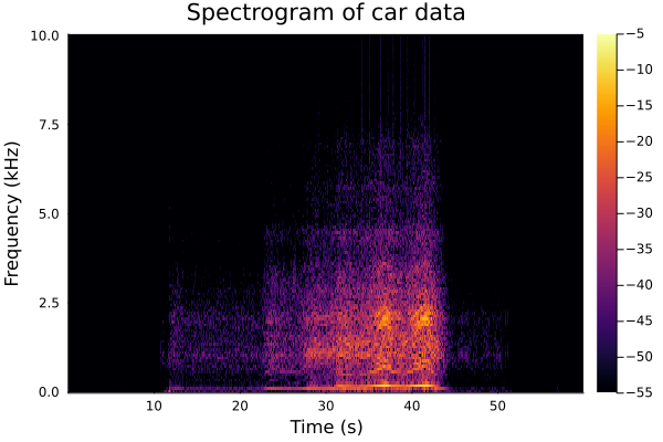
In the plot above, the $y$ -axis now corresponds to time and the $x$ -axis shows different frequency. The magnitude of the spectrum is depicted using different colors. This strategy of localization or windowing can also be used for constructing the DFT itself.

Spectral leakage

When performed on small time localized sections of the signal, the corresponding transform is often called the short-time-Fourier transform (STFT). This can be depicted mathematically as:

F(\tau, \omega) = \int \limits _{-\infty} ^{\infty} x(t) w (t - \tau) e^{-i \omega t} dt

where $w(t, \tau)$ is now a windowing function. However one should remember that the DFT expects the signal given to it to be periodic. When windowing, even for a periodic function, it is not necessary that the window applied contain an entire period (or integer multiple of the period) of the function as shown in the below plot. As a consequence, one gets a phenomenon termed spectral leakage but more on that in a bit.

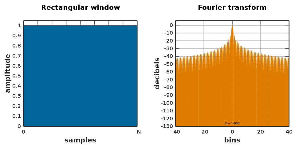
To force the function contained within the window to be periodic, it is common to taper both sides of the windowed portion to zero and this can be done in many ways. Thus, there are many choices for window functions and the Wikipedia page lists a litany of them. What one must remember though is that different window functions can lead to different characteristics in the magnitude spectrum output. These are easily visualized as shown below for a rectangular window function (from Wikipedia).

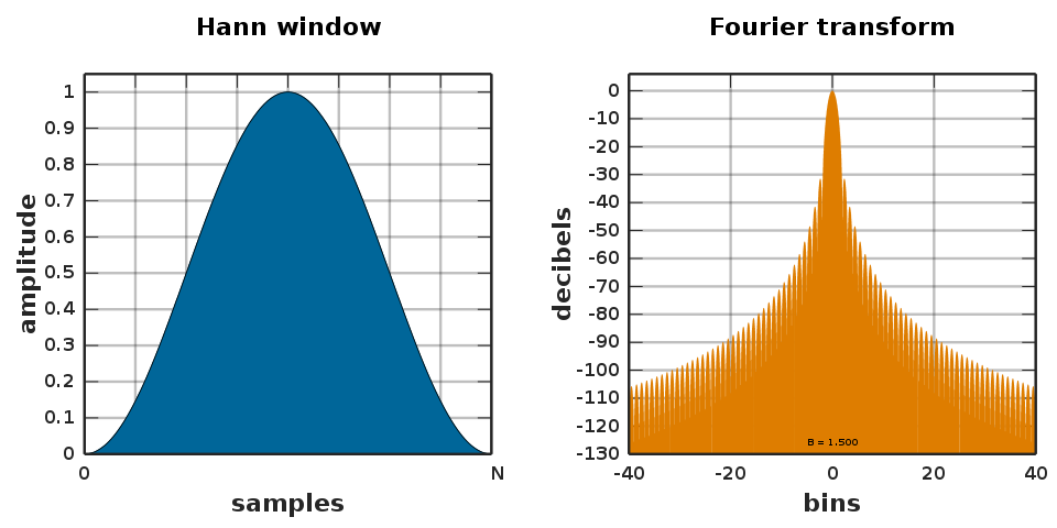
The next plot shows another popular window function called the Hann windows. In each case, the window functions are shown next to their FFT and one can see that leakage characteristics are different. In particular, if one were trying to distinguish two different frequency components, at -30 dB amplitude, then the second choice would be a better one.

To better understand what causes leakage, consider the cosine wave on the left below which has a window marked around it.

The plot on the right shows this windowed portion repeated to the left and the right - as seen by the DFT! Clearly, this function is repeating but there is an abrupt jump between the two "periods" and this explains the "leak". What tapering does is to force periodicity by driving the signal to zero at the beginning and the end. Therefore, while some choice of window function can reduce leakage, it cannot be gotten rid of entirely.

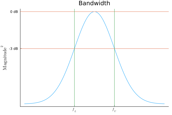
Bandwidth

Thus it seems like there is, in some sense, a "useful" portion of the frequency spectrum of a signal. This is often called the bandwidth. The precise definition is that the bandwidth of a signal is the frequency range within which the signal power drops to half its maximum magnitude. In log scale this is approximately -3dB.

Conclusion

In this lecture note we have discussed the effects of sampling on the DFT spectrum and the consequences of using the DFT when we should really be using the DTFT or CFT. Further, we discussed concepts like power spectral density, spectral leakage and bandwidth. The key points are:

The DFT is vulnerable to spectral leakage. Spectral leakage occurs when a non-integer number of periods of a signal is sent to the DFT. Spectral leakage lets a single-frequency signal be spread among several frequencies after the DFT operation. This makes it hard to find the actual frequency of the signal.
We can zero-pad the signal and perform a larger DFT to get a more frequency bins. Zero-padding a signal does not reveal more information about the spectrum, but it only interpolates between the frequency bins that would occur when no zero-padding is applied. In particular, zero-padding does not increase the spectral resolution.
To increase the spectral resolution, longer durations of real measurements are necessary. A longer measurement obtains more information from the measured signal, since the resulting frequency bins are distributed finer.
Different window functions have different characteristics and the choice depends on the application.

This brings us to the end of the first part of CSSB, which its author has termed Signals. In the next lecture we will start with analysis of systems in earnest.

[back]

[1]	As usual, good is in air quotes because it really depends on the application.

[2]	See spectral leakage

CC BY-SA 4.0 Ivan Abraham. Last modified: February 20, 2023. Website built with Franklin.jl and the Julia programming language. Curious? See familiar examples.