Lecture 04

Reading material: Section 2.2 & 2.4 of the textbook.

Recap

Last time we discussed the basic form of sinusoidal waveforms, some elementary transformations that can be performed on signals, derivation of Euler's formula that relates trigonometry with sinusoids and complex numbers as well as two main approaches to modeling of biological systems. Today we will continue discussing various methods of characterizing and analyzing statistics of signals as well as some specific waveforms commonly encountered in analysis.

Mean, variance, root-mean-square, etc.
The deciBel (dB)
Signal to noise ratio (SNR)
Some common waveforms
Correlation & covariance
1. Correlation
2. Covariance
Distance measures

Mean, variance, root-mean-square, etc.

This time we start discussing some ways to characterize the signals we will see in our work. The primary method of doing this will be by computing certain statistical properties and values of the signals. Consider the following to signals that show markedly different behaviors.

Consider the example of two signals shown in figure below:

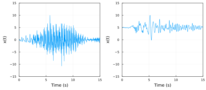
The two waveforms above display markedly different properties and behaviors.

The obvious difference is that one is oscillating around zero while the other is oscillating around the value 5. We could eliminate this difference by performing an elementary operation ( $y$ -axis shift) but closer inspection reveals that more is different: the one on the left seems to have "more energy" while the one on the right seems to be more "subdued".

Two properties that characterize these differences are the root-mean-square value (a.k.a RMS value) and variance both of which we can contrast with the mean. Recall the usual definitions.

Mean

For the mean value, we have two roughly equivalent definitions depending on whether the signal involved is discrete time or continuous time signals.

\mu _x = \dfrac{1}{N} \sum \limits _{n=1} ^{N} x_n \qquad \textrm{and} \qquad \mu _x = \dfrac{1}{T} \int \limits _0 ^T x(t) dt

While the mean characterizes the average value of a signal over its period of observation, the amount of fluctuation is measured by a term called variance defined as follows.

Variance & standard deviation

\sigma^2 = \dfrac{1}{N-1} \sum \limits _{n=1}^N \left( x_n - \mu _x \right)^2 \qquad \textrm{and} \qquad \sigma^2 = \dfrac{1}{T} \int \limits _0 ^T \left(x(t) - \mu _x \right) ^2 dt

The square root of the variance $\sigma ^2$ is defined to be the standard deviation $\sigma$ . Then it is easy to see that while the mean and standard deviation preserve the original units, the variance does not.

⚠️ Note

Keep in mind that the normalization is by

N-1

(denoting sample variance) and not

N

(used for population variance) which is a factor required to avoid biased estimates.

Root Mean Square

A quantity related to standard deviation is the root-mean-square value of a signal which has its origins in voltage and power calculations. This quantity is defined as:

x_{rms} = \left[ \dfrac{1}{N} \sum \limits _{n=1} ^N x_n^2 \right] ^{1/2} \qquad \textrm{and} \qquad x_{rms} = \left[ \dfrac{1}{T} \int \limits _0 ^T x(t)^2 dt \right] ^{1/2}

Traditionally when a signal was represented using a fluctuating voltage, the RMS value represented the constant voltage that would achieve the same power dissipation as the fluctuating one.

\begin{aligned} P = V(t)I = \dfrac{V(t)^2}{R} \quad &\implies \quad \bar{P} = \dfrac{1}{T} \int \limits _0 ^T \dfrac{V(t)^2}{R} dt = \dfrac{1}{R} \cdot \dfrac{1}{T} \int \limits _0 ^T V(t)^2 dt = \dfrac{V_{rms}^2}{R} \\ & \implies V_{rms} := \left[\dfrac{1}{T} \int \limits _0 ^T V(t)^2 dt \right]^{1/2} \end{aligned}

Thus the standard deviation is a term characterizing fluctuation about the mean whereas the RMS value is more of a statement about the essential magnitude of the signal.

The following table lists the RMS values of some periodic oscillatory waveforms with characteristic amplitude $A$ (i.e. the maximum and minimum amplitude is $\pm A$ ). In the case of periodic signals, it suffices to use Eq. (3) over one period and for symmetric periodic signals, the interval of integration can be even shorter.

Wave Type	RMS	Wave Type	RMS	Wave Type	RMS
Sine	$\dfrac{A}{\sqrt{2}}$	Square	$A$	Triangle	$\dfrac{A}{\sqrt{3}}$

Answer: Application of Eq. (3) results in:

\begin{aligned} y_{rms}^2 &= \dfrac{1}{T} \int \limits _0 ^T \left( A_0^2 + 2 A_0 A_1 \sin (\omega t) + A_1^2 \sin^2(\omega t) \right) dt \\ &= \dfrac{1}{T} \left[ \left. A_0^2t \right|_0^T + \left. \dfrac{2}{\omega} A_0 A_1 \cos (\omega t) \right|_0^T + A_1^2 \int \limits _0 ^T \left(\dfrac{1}{2} - \dfrac{\cos(2\omega t)}{2} \right) dt \right] \end{aligned}

The last term has been worked out in Example 2.1 of the textbook and the contribution from the first and middle terms are

A_0^2

and

0

respectively (make sure you work this out!). Thus,

y_{rms} = \sqrt{A_0^2 + \dfrac{A_1^2}{2}}

The deciBel (dB)

The decibel is a (rather arbitrary) "unit" used to compare the intensity or power level of a signal by comparing it against a reference signal on the logarithmic scale. Originally named after famed inventor Alexander Graham Bell, the Bel turned out to be too large unit to be useful and it is actually a tenth of its value (hence the "deci") that caught on. Given signal $V$ , when we compare it against a reference signal $V_0$ on the decibel scale, we express its intensity or amplitude as

V_{db} = 10 \log \left( \dfrac{V}{V_0} \right)

Defined as above the quantity $V_{db}$ has no units and represents a logarithm of a dimensionless ratio. A typical use then is to describe the signal-to-noise-ratio (SNR) of a signal as we will see in the following section. The logarithmic scale is useful when we want to express a wide range of values on the same graph and also has the added benefit of turning multiplication to addition in log units.

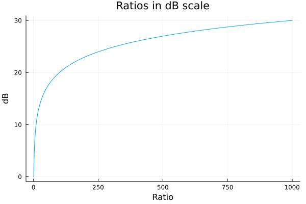
On the other hand, when decibels are used to characterize a single signal (taking reference $V_0=1$ ) then the units involved are written as dB Volts, dB dynes etc. to indicate this is the case. The figure below is a plot showing what ratios $\dfrac{V}{V_0}$ translate to decibels on the $y$ -axis. Here we can see that if $V$ is 100 times $V_0$ this translates to 20 dB whereas if $V$ is 1000 times $V_0$ the value is 30 dB.

In situations involving power calculations (where commonly a square term is involved) the decibel becomes

V_{db} = 10 \log \left( \dfrac{V^2}{V_0^2} \right) = 10 \log \left( \dfrac{V}{V_0} \right)^2 = 20 \log \left(\dfrac{V}{V_0} \right)

Signal to noise ratio (SNR)

The majority of waveforms are a mixture of signal and noise. Signal and noise are relative concepts, and depend on the work at hand: the signal is what you want from the waveform, whilst the noise is everything else. Therefore it is useful to characterize the level of each when analyzing a signal and thus SNR is defined as:

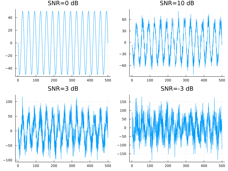
\operatorname{SNR} = 20 \log \left( \dfrac{\operatorname{signal}}{\operatorname{noise}} \right)

To develop intuition for SNR values, the following figure shows a noisy sinusoid of 30 Hz and 50 units amplitude at different levels of SNR.

Some common waveforms

We already saw examples of sine, square and triangle waves in the figures from Lecture 2. Here we discuss a few more along with the mathematical notations used to represent them.

Step signal

One of the simplest conceivable signals is one that is zero until a certain time $t_0$ and then takes on a constant value $c$ , after $t>t_0$ . We call such signals step signals. Mathematically we can write this as:

y (t) = \begin{cases} &0, \quad t < t_0 \\ &c,\quad t \geq t_0 \end{cases}

Since we are familiar with amplitude scalings time-axis shifts, it simplifies matters to write everything in terms of the unit step function $h(t)$ :

h(t) = \begin{cases} &0, \quad t <0 \\ &1, \quad t \geq 0 \end{cases}

Answer: We can write it as

c \cdot h(t-t_0)

Impulse signal

A special analytical (and idealized) signal defined and used for its ability to simplify concepts is the so-called impulse function defined by the following heuristic^[1]. The impulse function or Dirac delta function is one which satisfies

\delta(x) \approxeq \begin{cases} &\infty, \quad x = 0 \\ &0, \quad x \neq 0 \end{cases}

subject to the condition:

\int \limits _{\mathbb{R}} \delta(x) dx = 1

While it is not immediately obvious why such an abstraction should be useful, it might be useful to think about what the derivative of $h(t)$ above should be. We will see concrete examples of how the impulse function is used to simplify modeling in future lectures.

⚠️ Note

Technically, there is no mathematical "function" that satisfies the above property (see footnote) however one should think of it as a linear functional that maps every continuous function

f(x)

to its image at the origin

f(0)

Ramp signal

Speaking of derivatives of the unit step function; one is naturally motivated to think of what it's integral should be as well. The ramp function is mathematically defined as:

r(t) = \begin{cases} &0, \quad t < 0 \\ &t, \quad t \geq 0 \end{cases}

Exponential signal

While we have seen the exponential function in the context of Lecture 03, when talking of derivatives and integrals, the exponential function has yet another characterization as the function whose derivative is itself! Let's see this in action.

Solution: Let us proceed without an ansatz. The requirement is a function

f(x)

such that

f'(x) = f(x)

Actually more is true: the requirement is that any $n$ -th derivative $f^{(n)}(x) = f(x)$ . Thus this must be an infinitely differentiable function admitting a Taylor series $T_f (x) = \sum \limits _{k=0} ^{\infty} c_k x^k$ where the $c_k$ usually depend on successive derivatives but now are related via $f^{(n)}(x) = f(x)$ .

Differentiating the Taylor expansion once we get that a relationship must hold between the $c_k$ ; namely, _____ . For example, with $k=0$ we get $c_1 = c_0$ and $k=5$ we get $c_6 = \dfrac{c_5}{6}$ . A little recursion then gives that $c_k = \dfrac{c_0}{k!}$ . Thus the Taylor expansion becomes:

T_f(x) = \sum \limits _{k=0} ^ \infty c_0 \dfrac{x^k}{k!} = c_0 \sum \limits _{k=0} ^\infty \dfrac{x^k}{k!}

But the right hand side infinite sum should be familiar from calculus!. Thus we get the functions $y(x) = c_0 e^{x}$ are functions whose derivative satisfy $f(x) =f'(x)$ with $c_0$ being defined by $f(0)$ .

____ - Homework material.

Moreover, this characterization is unique; that is (upto some caveats) $ce^{x}$ are the only functions that equal their derivatives.

Solution: Assume there is another class of functions

g(x)

which are not of the form

g(x)=k e^{x}

such that

g'(y) = g(y)

. Now consider the derivative:

\left(g(x) e^{-x} \right)'

which by the product rule ____.

You will show in your homework the assumption leads to a contradiction. 😊

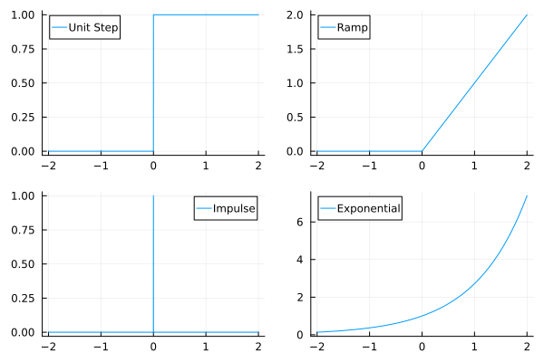
The figure below shows the three signals we have discussed so far:

Correlation & covariance

Given two signals, one natural question to ask is how similar are the signals? Can we associate some number or measure to a signal or a pair of signals that can tell us how similar they are? We have already defined the mean and variance for a signal. Thus one naturally asks if they are sufficient.

Solution: Left as an exercise.

As the answer to the above exercise shows, it is possible to have drastically different and mismatched signals that share the same mean and standard deviation but differ elementwise. The problem here is the mean and variance are properties of a single signal whereas for similarity we need to look at both signals.

Enter correlation.

Correlation

In words, two correlated signals exhibit behavior that seem in tandem with each other; i.e. they may increase or decrease at the same time. Consider the two figures:

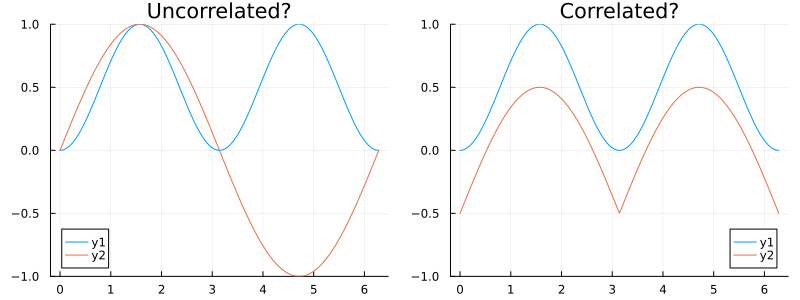
It is clear that two signals on the right pane move in tandem while the situation is less clear for the pair on the left. Mathematically we capture this essential observation via the following definition: the Pearson correlation coefficient between two sampled signals $x$ and $y$ is given as

r_p(x, y) = \dfrac{1}{N-1} \sum \limits _{k=1} ^N \left( \dfrac{x_k - \mu _x}{\sigma _x} \right) \cdot \left(\dfrac{y_k - \mu _y}{\sigma _y} \right)

which is a quantity restricted to be between $-1$ and $1$ with either value representing perfect linear anti-correlation or correlation and the middle value (zero) implying no correlation. Note the normalization by $N-1$ for sample statistics similar to the definition for variance.

Answer: Let

\bar{x} = x - \mu _x

and similarly

\bar{y} = y - \mu _y

to be the mean centered version of

x

and

y

. Consider

r(x, y) = \dfrac{1}{N} \sum \limits _{k=1} ^N \left( \dfrac{x_k - \mu _x}{\sigma _x} \right) \cdot \left(\dfrac{y_k - \mu _y}{\sigma _y} \right)

so that

r = r_p \cdot \dfrac{N-1}{N}

(thus

r < r_p

with a bit of handwaving since we are switching to population and not sample statistics above). Now note,

r(x, y) = \dfrac{1}{N} \sum \limits _{k=1} ^N \dfrac{\bar{x}_k \cdot \bar{y}_k}{\sigma _x \cdot \sigma _y} = \dfrac{1}{N} \cdot \dfrac{\bar{x} ^T \bar{y}}{ \sigma_x \sigma_y}

but

\sigma _x^2 = \dfrac{1}{N} \sum \limits _{k=1} ^N \bar{x}_k^2 = \dfrac{1}{N} \bar{x}^T \bar{x} = \dfrac{1}{N} \|\bar{x}\|^2

. Thus,

r(x, y) = \dfrac{\bar{x}^T \bar{y}}{\|x\|\|y\|}

Thus $r(x, y)$ is the dot product of two unit vectors; and thus equal to the cosine of the "angle" (in whatever number of dimensions) between them; and thus restricted between $-1$ and $1$ which then carries over to $r_p$ .

Covariance

When written absent the normalization factor, we get the covariance between two vectors:

\operatorname{cov}(x, y) = \dfrac{1}{N-1} \sum \limits _{k=1} ^N (x_k - \mu _x) \cdot (y_k - \mu _y)

Often people also use the term "correlation" to refer to an un-normalized correlation, especially in the context of continuous time signals:

r(x, y) = \dfrac{1}{T} \int \limits _0 ^T x(t) y(t) dt

Be sure to read Section 2.4.1 of CSSB for details!!

Distance measures

While in the above we discussed correlation and covariance, which measure how much signals vary together, it turns out that it is quite useful to have a measure of "distance" (akin to real life Euclidean distance) between objects (in this case signals) of interest in whichever mathematical space we are working in. This then allows all sorts of maximization/minimization etc. Mathematically what we need is a function $f$ satisfying the following: given $x, y$ two signals,

$f(x, y) = f(y, x)$
$f(x, y) > 0$ for all $x \neq y$ and $f(x, y) = 0$ if and only if $x = y$ .
$f(x, z) \leq f(x, y) + f(y, z)$

The last requirement is not obvious; but is a desirable property to have for a natural notion of distance (e.g. stopping at the grocery on the way home should naturally take more time than going straight home). Functions that do not satisfy all the above requirements are not called true metrics and are sometimes referred to as pseudo-metrics.

Answer: It is indeed an exercise and might show up in your homeowork.

[back]

[1]	It is a heuristic because a mathematically rigorous definition of the Dirac function necessitates the invocation of measure theory or the theory of distributions.

CC BY-SA 4.0 Ivan Abraham. Last modified: February 05, 2023. Website built with Franklin.jl and the Julia programming language. Curious? See familiar examples.