Homework 3 - Due: 02/08

Problem 1

Consider the following matrices:

\[ A_1 = \begin{bmatrix} 1/2 & -1/2 \\ 1/2 & -1/2 \end{bmatrix}, \qquad A_2=\begin{bmatrix}0&1\\-1&0\end{bmatrix},\qquad A_3=\begin{bmatrix}1&0&0\\0&-2&0\\-3&0&-2\end{bmatrix}. \]

  1. Compute \(e^{A_i t}\) for \(i=1,2,3\). Note that \(A_2\) is a special case of a matrix whose exponential was computed in class.
  2. For \(i=1,2,3\), write down the solution of \(\dot x=A_i x\) for a general initial condition.
  3. In each case, determine whether the solutions of \(\dot x=A_i x\) decay to 0, stay bounded, or go to \(\infty\) (for various choices of initial conditions).
  4. Try to state the general rule which can be used to determine, by looking at the eigenstructure of \(A\), whether the solutions of \(\dot x=A x\) decay to 0, stay bounded, or go to \(\infty\).

Problem 2

The pictures in this demo page show possible trajectories of a linear system \(\dot x= Ax\) in the plane, when the eigenvalues \(\lambda_1\) and \(\lambda_2\) of \(A\) are in one of the following six configurations:

# Configuration # Configuration
(a) \(\lambda_1<\lambda_2<0\) (b) \(\lambda_1<0<\lambda_2\)
(c) \(0<\lambda_1<\lambda_2\) (d) \(\lambda_1,\lambda_2=a\pm ib, \; a<0\)
(e) \(\lambda_1,\lambda_2=a\pm ib, \; a=0\) (f) \(\lambda_1,\lambda_2=a, \; a>0\)

Match each picture with the corresponding eigenvalue distribution. Justify your answers using your knowledge of the solution of \(\dot x = Ax\). Plotting in MATLAB or use of the demo applet cannot be used as a justification.
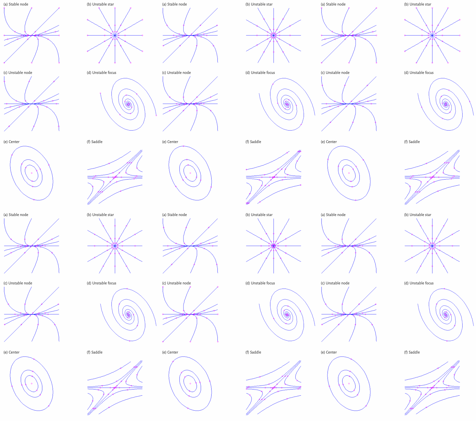
Animations courtesy of Prof. R.B. Israel

Problem 3

This exercise illustrates the phenomeom known as resonance. Consider the system

\[\begin{align*} \begin{bmatrix} \dot x_1\\ \dot x_2 \end{bmatrix} &= \begin{bmatrix} 0 & \omega \\ -\omega & 0 \end{bmatrix} \begin{bmatrix} x_1\\ x_2 \end{bmatrix} +\begin{bmatrix} 0\\ 1 \end{bmatrix}u,\qquad y=x_2 \end{align*}\]

where \(\omega>0\), \(u\) is the control input, and \(y\) is the output. Let the input be \(u(t)=\cos\nu t\), \(\nu>0\). Using the variation-of-constants formula, compute the response \(y(t)\) to this input from the zero initial condition \(x(0)=0\), considering separately two cases: \(\nu\ne\omega\) and \(\nu=\omega\). In each case, determine whether this response is decaying to 0, bounded, or unbounded.

Problem 4

Compute the state transition matrix \(\Phi(t,t_0)\) of \(\dot x=A(t)x\) with \[A(t) = \begin{bmatrix}-1+\cos t&0 \\0&-2+\cos t \end{bmatrix}\]

Problem 5

Consider the LTV system \(\dot x=A(t)x\), where \(A(t)\) is periodic with period \(T\), i.e., \(A(t+T)=A(t)\). Let \(\Phi(t,t_0)\) denote the corresponding state transition matrix. The goal of this exercise is to show that we can simplify the system and characterize its transition matrix with the help of a suitable (time-varying) coordinate transformation.

Being a nonsingular matrix, \(\Phi(T,0)\) can be written as an exponential: \(\Phi(T,0)=e^{RT}\), where \(R\) is some (possibly complex-valued) matrix. Define also:

\[P(t):=\Phi(t,0)e^{-Rt}\]

  1. Using the properties of state transition matrices from class, show that \(\Phi(t,t_0)=P(t)e^{R(t-t_0)}P^{-1}(t_0).\)
  2. Deduce from a) that \(\bar x(t):=P^{-1}(t)x(t)\) satisfies the time-invariant differential equation \(\dot{\bar x}=R\bar x\).
  3. Prove that \(P(t)\) is periodic with period \(T\).
  4. Consider the LTV system from Problem 4 . Find new coordinates \(\bar x(t)\) in which, according to part b), this system should become time-invariant. Confirm this fact by differentiating \(\bar x(t)\).

Problem 6

Prove the variation-of-constants formula for linear time-varying control systems stated in class: \[ x(t) = \phi(t,t_0)x_0 + \int \limits _{t_0} ^{t} \phi \left(t, s \right) B(s) u(s) ds \] satisfies the LTV controlled systems’ differential equation.

Hint: Differentiate both sides. See also Class Notes, end of Section 3.7.