For students who intend to scribe, you can see the source code for this page by clicking the code button above this callout. The source is compatible with the Quarto publishing system.
Scribed by: itabrah2
Introduction
This course is titled “Control System Theory & Design”. Let us start by first asking what we mean by a system; after all, it is a word used in many different contexts and with different meanings. For our purposes, a system is a collection of interrelated processes and/or signals that, together, achieve some objective. For example, the circulatory system’s objective is to ensure oxygenated blood from the lungs reaches all parts of the human body and, remove CO2 from different parts of the body and transfer it to the lungs. Similarly, the HVAC system’s objective is to maintain a comfortable ambiance for the occupants of a building by controlling factors like humidity and temperature.
A control system is one in which a certain subcollection of signals and processes direct, control, command and/or regulate other processes. Recall that in classical control, we had a plant model where a system with output took input , which a controller determined - often by comparison against a reference signal . An example we are familiar with is cruise control in an automobile, where a sensor measures the wheel velocity and, by comparison to the set or desired velocity, determines the appropriate amount of fuel or throttle to be provided (the control signal).
Unity feedback configuration
In this course, the object of study is control systems, which can be considered a generalization of classical dynamical systems (a control system with no inputs typically reduces to a dynamical system). What is different from classical controls course here is the shift in focus from the frequency domain to the time domain. In prior courses, we avoided dealing with differential equations by taking the Laplace transform and moving to the complex frequency domain. In this course, we will focus more on the ODEs and study them in detail, especially in the context of linear systems.
To illustrate what we mean, consider the following systems:
An object in free fall
A pendulum
An RC circuit
and their so called equations of motion.
An object in free fall
Object in free fall
Suppose the object has mass and experiences acceleration . For this simplified model we will only consider the effect of gravity and aerodynamic drag (assume proportional to velocity). By Newton’s second law, we must have the net sum of all forces acting on a free-falling object equal its mass times acceleration. Thus,
where is a term that retards the downward motion of the object (i.e. drag force).
A pendulum
Consider the case of a pendulum of length and mass (connected to its base by a massless string) subtending an angle . In this case, when we apply Newton’s second law seperately to the tangential and radial axes we see that radial components cancel. On the other hand, the equation describing the tangential component gives us:
Pendulum in swing
However, the angle is related to the arclength subtended as where is the arclength. Then and
An RC circuit
RC circuit
For an RC circuit with current under an external voltage supply we can write Kirchoff’s Voltage Law as:
where is the voltage across the capacitor. However, we know that is the governing equation for the capacitor of capacitance where is the charge in the capacitor. Differentiating we get except the current. Thus,
At this point we have looked at an electrical system, an aerodynamical example and a mechanical system.
All of these are differential equations of the form where and . In other words is some function that consumes a vector and returns another vector .
The majority of this course is concerned with systems of the form(s):
sometimes written with an explicit time dependence as
The latter systems are called non-autonomous systems while the former are called autonomous systems. In either case, (autonomous or non-autonomous), the second variety (involving or ) indicates the presence of an input term and so signifies a control system (we usually consider the input term to be some form of control law).
Tip
Note that in and its siblings, the left-hand-side (LHS) consists of a single (if vector valued) term that is a first derivative whereas the right-hand-side (RHS) has no derivatives at all. This form is usually called the standard state-space formulation. Each entry of is a state variable and collectively captures the state of the system - information that fully determines all aspects of a system at a particular instant of time and along with any initial conditions, sufficient to predict all future states.
where the second term involving can be considered the input into the system. The other two require a tad bit more algebra. Let us come back to it after we discuss some course logistics.
For the purposes of this class linear systems are ones in which we can write or as where the matrices and are devoid of any state variables.
Example: We can write
as
Question: standard drag force
In the example of the free falling body we considered, the drag experienced by the falling object was directly proportional to its velocity. In reality, the drag force increases drastically with changes in velocity and we often model it as quadratic in velocity. Is such a system linear or nonlinear?
The linear state space formulation
Generally, in a physical system that we week to influence we do not have access to all state variable. In other words, though a phenomenon may involve variables, which together completely determine the state vector, one may only be able to observe some variables which may either be the state variables themselves or a linear combination thereof. We represent this situation by writing:
or
In the above is a matrix, of size , and of dimension . They are typically called the system, input and output matrices. The matrix captures any direct influence the input has on the output .
Note about the feed-through matrix
We will see how the matrix arises when we discuss the relation between the state-space formulation and transfer functions.
Though we remarked that the we will focus on the time domain description in this course, and we will discuss realization theory in greater detail at a later time, it is now instructive to examine what happens if we simply take the Laplace transform of Equation 4. For simplicity assume . We get
Isolating from the first, plugging it into the second and rearranging we get
which provides a means to convert a given state-space model into its transfer function model.
Caution
In the above we made the assumption . This results in a single-input and single-output (SISO) model and the matrix necesarily reduces to a scalar entity . Equation 5 is only valid in this case. For the general MIMO (multi-input multi-output) case, what we end up having is a transfer function matrix. In other words, a transfer function between each pair of inputs and outputs.
Question: Given a transfer function how do we find the corresponding state-space model? Is this model unique?
It turns out that there are many ways to generate a state-space model from the transfer function and they result in slightly different (but equivalent) formulations in terms of the matrices . To truly appreciate why this happens, we need to review some linear algebra material. Such material will be the focus of the next few lectures.
However, before that we review some systems concepts.
Linearity
From prior courses, we are familiar with the input-output description of a linear system:
which reduces to a convolution for time invariant systems. Let us make precise what we mean by linear and time invariant.
Definition 1 (Linearity) A function is linear . In terms of systems, a system is said to be linear if for any two state-input pairs
mapping to outputs and , i.e. we have that,
In other words, if the states and inputs are scaled and added then the resultant output is also a scaled and added version of individual outputs.
Addition here is interpreted pointwise in time.
If the input to a system is zero then the system response starting from some initial condition is caleld the zero-input response. If the system starts from a zero initial condition and evolves under some input , the system response is called the zero-state response.
An important property of linear systems is that the response of any system can be decomposed into the sum of a zero-state reponse and a zero-input response.
Tip
Verify the above statement directly follows from the linearity property.
Additionally, a system is said to be lumped if the state vector necessary to describe it is finite dimensional. A system is said to be causal if the current output only depends on the past inputs to the system and not on any future input. We will exclusively deal with lumped causal systems in this course.
If we deal with continuous time systems and if then we say we deal with discrete time systems. The results we derive will primarily be for continous time systems and occassinally for discrete time systems. LSTC does a parallel treatment of both time-invariant and time-varying systems so you are encouraged to read it as supplementary material. When we do deal with discrete time systems, we will assume that the sampling period is uniform.
Time invariance
A special class of systems where our study can be made much deeper is the class of linear time invariant systems.
Definition 2 (Time invariance) A system is said to be time invariant if for every initial state & input-output pair, and any , we have,
In other words, starting from the same initial condition, a time shift of the input function by an amount results in a time shift of the output function by the same amount. Thus for linear time invariant systems (LTI), we can assume with no loss of generality that .
Why is one argument and the other ?
Be sure to understand this point about notation. The expression: should be interpreted as initial condition at time (written as ) under the action of (for ) results in output . Thus,
should be interpreted as initial condition at time under the action of the time shifted input (for ) gives rise to output .
Transfer functions
Above we saw the relationship between the state-space (SS) formulation and the transfer function via the Laplace transform. Before we proceed to a review of some concepts from linear algebra, it is a good idea to review some frequency domain concepts. Let us use to denote the degree of some polynomial .
For lumped systems, transfer functions are rational functions, i.e. can be written as a polynomial divided by another polynomial:
If then a transfer function is said to be proper.
If then a transfer function is said to be strictly proper.
If then a transfer function is said to be bi proper.
Finally, a complex variable is said to be a pole of a rational transfer function if and a zero if .
If and are co-prime, i.e. do not share any common factors of degree 1 or higher, then all roots of are zeros and all roots of are poles.
Course overview
At the heart of all control systems are dynamical systems and dynamical systems essentially boil down to differential or difference equations. Our prior treatment of control systems was algebraic in some sense because we sidestepped dealing with ODEs by applying the Laplace transform and going to the complex frequency domain. We made significant progress in studying such systems by developing tools like the Root Locus method, Bode plots, Nyquist criterion, etc. Nevertheless, these are called classical control techniques (as opposed to modern control theory) because, in a certain sense (the precise sense of which will hopefully become more apparent by the end of the course), the state-space formulations offer a richer characterization. In this sense, one may call the state-space formulation a more geometric approach, and to proceed, we will make ample use of linear algebraic techniques. The rest of the course will proceed as follows:
Linear algebra review (part 1)
Linear systems and their solutions
Linear algebra review (part 2)
Stability of dynamical and control systems
Controllability - what can we control about a system?
Observability - what can we know about a system from observations?
Realization theory (bridge transfer functions & SS formulation)
Feedback control - SS perspective
Pole placement and observer design
Observer-based feedback
Optimal control concepts
Source Code
---Title: Lecture 01 - 01/16code-tools: source: true toggle: false---::: {.callout-note}For students who intend to scribe, you can see the source code for this pageby clicking the code button above this callout. The source is compatible with the[Quarto](https://quarto.org/) publishing system. Scribed by: _itabrah2_:::## IntroductionThis course is titled "_Control System Theory & Design_". Let us start by firstasking what we mean by a **system**; after all, it is a word used in manydifferent contexts and with different meanings. For our purposes, a system is acollection of interrelated processes and/or signals that, together, achievesome objective. For example, the circulatory system's objective is to ensureoxygenated blood from the lungs reaches all parts of the human body and, removeCO2 from different parts of the body and transfer it to the lungs. Similarly,the HVAC system's objective is to maintain a comfortable ambiance for theoccupants of a building by controlling factors like humidity and temperature.A **control system** is one in which a certain subcollection of signals andprocesses direct, control, command and/or regulate other processes. Recall that inclassical control, we had a plant model where a system with output $y$ tookinput $u$, which a controller determined - often by comparison against areference signal $r$. An example we are familiar with is cruise control in anautomobile, where a sensor measures the wheel velocity and, by comparison tothe set or desired velocity, determines the appropriate amount of fuel orthrottle to be provided (the control signal). {width=60%}In this course, the object of study is _control systems_, which can beconsidered a generalization of classical dynamical systems (a control systemwith no inputs typically reduces to a dynamical system). What is different fromclassical controls course here is the shift in focus from the frequencydomain to the time domain. In prior courses, we avoided dealing withdifferential equations by taking the Laplace transform and moving to thecomplex frequency domain. In this course, we will focus more on the ODEs andstudy them in detail, especially in the context of _linear systems_.To illustrate what we mean, consider the following systems: - An object in free fall - A pendulum - An RC circuit and their so called equations of motion. #### An object in free fall ::: {.column-margin}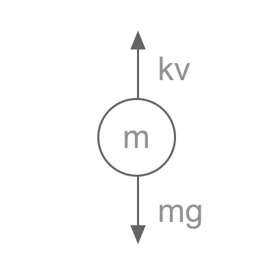{width=60%}:::Suppose the object has mass $m$ and experiences acceleration $a$. For thissimplified model we will only consider the effect of gravity and aerodynamicdrag (assume proportional to velocity). By Newton’s second law, we must havethe net sum of all forces acting on a free-falling object equal its mass timesacceleration. Thus,$$ mg - kv = ma$$ {#eq-1}where $kv$ is a term that retards the downward motion of the object (i.e. dragforce). #### A pendulum Consider the case of a pendulum of length $l$ and mass $m$ (connected to itsbase by a massless string) subtending an angle $\theta$. In this case, when weapply Newton's second law seperately to the tangential and radial axes we seethat radial components cancel. On the other hand, the equation describing thetangential component gives us:::: {.column-margin}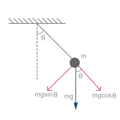{width=90%}:::$$ F = ma \quad \implies \quad -mg \sin \theta = ma $$ However, the angle $\theta$ is related to the arclength subtended as $s = l\theta$ where $s$ is the arclength. Then $\ddot a = l \ddot \theta$ and $$ \ddot{\theta} + \dfrac{g}{l} \sin\theta = 0 $$ {#eq-2}#### An RC circuit ::: {.column-margin}{width=80%}:::For an RC circuit with current $I$ under an external voltage supply $V$ we canwrite Kirchoff's Voltage Law as:$$ V = IR + V_c $$where $V_c$ is the voltage across the capacitor. However, we know that $q =CV_c$ is the governing equation for the capacitor of capacitance $C$ where $q$is the charge in the capacitor. Differentiating we get $\dot{q} = C\dfrac{dV}{dt}$ except $\dot q = I$ the current. Thus, $$ V = RC\dot{V_c} + V_c$$ {#eq-3}At this point we have looked at an electrical system, an aerodynamical exampleand a mechanical system. ::: {.callout-caution collapse="true"}## What is common to @eq-1, @eq-2 and @eq-3? All of these are **differential equations** of the form $\dot x = f(x)$ where $x\in \mathbb{R}^n, n\ge 1$ and $f: x \mapsto \mathbb{R}^n$. In other words $f$is some function that consumes a vector $x$ and returns another vector $f(x)$. ::: The majority of this course is concerned with _systems_ of the form(s):$$\dot x = f(x) \qquad \textrm{and} \qquad \dot x = f(x, u)$$sometimes written with an explicit time dependence as$$\dot x = f(t, x(t)), \qquad \textrm{and} \qquad \dot x = f(t, x(t), u(t)) $$The latter systems are called _non-autonomous_ systems while the former arecalled _autonomous_ systems. In either case, (autonomous or non-autonomous), thesecond variety (involving $u$ or $u(t)$) indicates the presence of an _input_ term$u, u(t) \in \mathbb{R}^p$ and so signifies a control system (we usuallyconsider the input term to be some form of control law). ::: {.callout-tip}Note that in $\dot x = f(x)$ and its siblings, the left-hand-side (LHS) consistsof a single (if vector valued) term that is a _first derivative_ whereas theright-hand-side (RHS) has no derivatives at all. This form is usually calledthe standard **state-space formulation.** Each entry of $x$ is a state variableand $x$ collectively captures the _state_ of the system - information thatfully determines all aspects of a system at a particular instant of time andalong with any initial conditions, sufficient to predict all future states. :::**Claim:** Each of @eq-1, @eq-2, @eq-3 can be written in the form: $\dot x = f(x, u)$. For @eq-3 we have by simple re-arrangement$$\dot V_c = \dfrac{1}{RC}V_c + \dfrac{1}{RC} V$$where the second term involving $V$ can be considered the input into thesystem. The other two require a tad bit more algebra. Let us come back to itafter we discuss some course logistics. ---> Break to discuss: [https://courses.grainger.illinois.edu/ece515/sp2024](https://courses.grainger.illinois.edu/ece515/sp2024)---For @eq-2, we had:$$mg - kv = ma \quad \implies \quad a = \dfrac{-k}{m}v + g$$However, $a = \dot v$ and $v = \dot y$ where $y$ is the downward displacement.Define auxilliary variables $z_1 =y$ and $z_2 = \dot y$. Then $\dot z_2 = \ddoty$ and $\dot z_1 = z_2$. Thus we get, $$\begin{align}\dot z_1 &= z_2 \\\dot z_2 &= \dfrac{-k}{m} z_2 + g\end{align}$$Now this is a two-dimensional system because $z = \begin{bmatrix} z_1 &z_2\end{bmatrix}^T \in \mathbb{R}^2$. For @eq-3, similarly, we had:$$\ddot \theta = -\dfrac{g}{l} \sin \theta $$Here we define, $x_1 = \theta$ and $x_2 = \dot x_1$. Then, we get, $$\begin{align} \dot x_1 &= x_2 \\ \dot x_2 &= -\dfrac{g}{l} \sin x_1 \end{align}$$### Linear vs. nonlinear system While we have written each of @eq-1, @eq-2 and @eq-3 in the standard statespace (SS) form, there is something special about @eq-3. In fact, @eq-1 and@eq-2 are _linear_ equations whereas @eq-3 is a _nonlinear_ equation. For the purposes of this class _linear_ systems are ones in which we can write$\dot x = f(x, u)$ or $\dot x = f(t, x(t), u(t))$ as $$\dot x = Ax + Bu \quad \textrm{or} \quad \dot x = A(t)x + B(t) u $$where the matrices $A$ and $B$ are devoid of any state variables. **Example:** We can write $$\begin{align}\dot z_1 &= z_2 \\\dot z_2 &= \dfrac{-k}{m} z_2 + g\end{align}$$as $$\dot z = \begin{bmatrix} 0 &1 \\ 0 & -k/m \end{bmatrix}z + \begin{bmatrix} 0\\1 \end{bmatrix} g \qquad \textrm{where} \quad z = [z_1 \; z_2]^T$$::: {.callout-caution}### Question: standard drag force In the example of the free falling body we considered, the drag experienced bythe falling object was directly proportional to its velocity. In reality, thedrag force increases drastically with changes in velocity and we often model itas quadratic in velocity. Is such a system linear or nonlinear? :::## The linear state space formulation Generally, in a physical system that we week to influence we do not have accessto all state variable. In other words, though a phenomenon may involve $n$variables, which together completely determine the state vector, one may onlybe able to observe some $q<n$ variables which may either be the state variablesthemselves or a linear combination thereof. We represent this situation bywriting:$$\begin{align}\dot x &= Ax + Bu \\y &= Cx + Du \end{align} $$ {#eq-4}or $$\begin{align}\dot x &= A(t)x + B(t)u \\y &= C(t)x + D(t) u \end{align}$$In the above $A$ is a $n\times n$ matrix, $B$ of size $n \times p$, and $C$ ofdimension $q \times n$. They are typically called the system, input and outputmatrices. The matrix $D$ captures any _direct_ influence the input $u$ has onthe output $y$. ::: {.callout-tip}### Note about the feed-through matrix We will see how the $D$ matrix arises when we discuss the relation between thestate-space formulation and transfer functions.:::Though we remarked that the we will focus on the time domain description inthis course, and we will discuss _realization_ theory in greater detail at alater time, it is now instructive to examine what happens if we simply take theLaplace transform of @eq-4. For simplicity assume $p=q=1$. We get$$s X(s) = AX(s) + BU(s) \qquad \textrm{and} \qquad Y(s) = CX(s) + d \cdot U(s) $$Isolating $X(s)$ from the first, plugging it into the second and rearranging we get $$G(s):= \dfrac{Y(s)}{U(s)} = C \left(sI - A \right)^{-1}B + d $$ {#eq-5}which provides a means to convert a _given_ state-space model $\left(A, B, C,D\right)$ into its transfer function model. ::: {.callout-caution}In the above we made the assumption $p=q=1$. This results in a single-input andsingle-output (SISO) model and the $D$ matrix necesarily reduces to a scalarentity $d$. @eq-5 is only valid in this case. For the general MIMO (multi-inputmulti-output) case, what we end up having is a _transfer function matrix_. Inother words, a transfer function between _each pair_ of inputs and outputs. :::**Question:** Given a transfer function how do we find the correspondingstate-space model? Is this model unique? It turns out that there are many ways to generate a state-space model from thetransfer function and they result in slightly different (but equivalent)formulations in terms of the matrices $(A, B, C, D)$. To truly appreciate why thishappens, we need to review some linear algebra material. Such material will bethe focus of the next few lectures. However, before that we review some systems concepts. ### Linearity From prior courses, we are familiar with the input-output description of a_linear system_:$$y(t) = \int \limits _{t_0} ^{t} G(t, \tau) u(\tau) d \tau $$which reduces to a convolution for _time invariant_ systems. Let us makeprecise what we mean by _linear_ and _time invariant_. ::: {#def-linear}## Linearity <br>A function $f$ is linear $f(\alpha x + y ) = \alpha f(x) + f(y)$. In terms ofsystems, a system is said to be linear **if** for any two state-input pairs$$(x_1(t_0), u_1(t)) \quad \textrm{and} \quad (x_2(t_0), u_2(t))$$ mapping to outputs $y_1(t)$ and $y_2(t)$, i.e. $$(x_1(t_0), u_1(t)) \mapsto y_1(t)) \qquad \textrm{and} \qquad (x_2(t_0),u_2(t)) \mapsto y_2(t)$$we have that, $$(x_1(t_0) + \alpha x_2(t_0), u_1(t) + \alpha u_2(t)) \quad \mapsto \quad y_1(t)+ \alpha y_2(t)$$:::In other words, if the states and inputs are scaled and added then theresultant output is also a scaled and added version of individual outputs. ::: {.column-margin}Addition here is interpreted _pointwise_ in time. :::If the input to a system is zero then the system response starting from someinitial condition $x_0 = x(t_0)$ is caleld the _zero-input_ response. If thesystem starts from a zero initial condition and evolves under some input$u(t)$, the system response is called the _zero-state_ response. An important property of linear systems is that the response of any system canbe decomposed into the sum of a zero-state reponse and a zero-input response. $$\textrm{response} = \textrm{zero-state response} + \textrm{zero-input response}$$::: {.callout-tip}Verify the above statement directly follows from the linearity property. :::Additionally, a system is said to be **lumped** if the state vector necessaryto describe it is finite dimensional. A system is said to be **causal** if thecurrent output only depends on the past inputs to the system and not on anyfuture input. We will exclusively deal with _lumped causal systems_ in thiscourse. If $t \in \mathbb{R}$ we deal with **continuous time** systems and if $t \in\mathbb{Z}$ then we say we deal with **discrete time** systems. The results wederive will primarily be for continous time systems and occassinally fordiscrete time systems. LSTC does a parallel treatment of both time-invariantand time-varying systems so you are encouraged to read it as supplementarymaterial. When we do deal with discrete time systems, we will assume that thesampling period is uniform. ### Time invariance A special class of systems where our study can be made much deeper isthe class of linear _time invariant_ systems. ::: {#def-timeinvariant}## Time invariance <br>A system is said to be **time invariant** if for every initial state &input-output pair, $$(x(t_0), u(t)) \mapsto y(t)$$and any $T$, we have, $$(x(t_0 + T), u(t - T)) \mapsto y(t - T)$$In other words, starting from the same initial condition, a time shift of the inputfunction by an amount $T$ results in a time shift of the output function by thesame amount. Thus for linear time invariant systems (LTI), we can assume withno loss of generality that $t_0=0$. :::::: {.callout-caution collapse="true"}## Why is one argument $t_0 + T$ and the other $t-T$? Be sure to understand this point about notation. The expression:$$(x(t_0), u(t)) \mapsto y(t)$$ should be interpreted as initial condition $x$ at time $t_0$ (written as$x(t_0)$) under the action of $u(t)$ (for $t>t_0$) results in output $y(t)$.Thus, $$(x(t_0 + T), u(t - T)) \mapsto y(t - T)$$should be interpreted as initial condition $x$ at time $t_0 + T$ under theaction of the time shifted input $u(t-T)$ (for $t>t_0 + T$) gives rise tooutput $y(t-T)$. :::### Transfer functions Above we saw the relationship between the state-space (SS)formulation and the transfer function via the Laplace transform. Before weproceed to a review of some concepts from linear algebra, it is a good idea toreview some frequency domain concepts. Let us use $\deg(P)$ to denote the_degree_ of some polynomial $P(s)$. * For lumped systems, transfer functions are rational functions, i.e. can be written as a polynomial divided by another polynomial: $$G(s) = N(s)/D(s)$$ * If $\deg(N) <= \deg(D)$ then a transfer function is said to be _proper._ * If $\deg(N) < \deg(D)$ then a transfer function is said to be _strictly proper._ * If $\deg(N) = \deg(D)$ then a transfer function is said to be _bi proper._Finally, a complex variable $\lambda$ is said to be a **pole** of a rationaltransfer function $G(s)$ if $|G(\lambda)|= \infty$ and a **zero** if $|G(\lambda)| = 0$. If $N(s)$ and $D(s)$ are _co-prime_, i.e. do not share anycommon factors of degree 1 or higher, then all roots of $N(s)$ are zeros andall roots of $D(s)$ are poles. ## Course overview At the heart of all control systems are dynamical systems and dynamical systemsessentially boil down to differential or difference equations. Our priortreatment of control systems was algebraic in some sense because we sidesteppeddealing with ODEs by applying the Laplace transform and going to the complexfrequency domain. We made significant progress in studying such systems bydeveloping tools like the Root Locus method, Bode plots, Nyquist criterion,etc. Nevertheless, these are called classical control techniques (as opposed tomodern control theory) because, in a certain sense (the precise sense of whichwill hopefully become more apparent by the end of the course), the state-spaceformulations offer a richer characterization. In this sense, one may call thestate-space formulation a more geometric approach, and to proceed, we will makeample use of linear algebraic techniques. The rest of the course will proceedas follows: * Linear algebra review (part 1) * Linear systems and their solutions * Linear algebra review (part 2) * Stability of dynamical and control systems * Controllability - what can we control about a system? * Observability - what can we know about a system from observations? * Realization theory (bridge transfer functions & SS formulation) * Feedback control - SS perspective * Pole placement and observer design * Observer-based feedback * Optimal control concepts


