ECE 486 Control Systems
Lecture 7
Effect of Extra Zeros
We discussed transient response characteristics last time, specifically rise time \(t_r\), overshoot \(M_p\) and settling time \(t_s\). We also sketched possible pole locations when there are constraints on them.
In this lecture, we will try to understand the effect of zeros and high-order poles on the shape of transient response, then its relation with stability. Following this line, we will formulate and learn how to apply the Routh–Hurwtiz stability criterion in the second half of this lecture.
Recall a system transfer function is a rational function \[H(s) = \dfrac{q(s)}{p(s)},\] its zeros are the roots of the numerator polynomial equation \(q(s) = 0\).
Extra Zero on Left Half Plane
Example 1: Consider transfer function \(H_1(s)\) with normalized natural frequency \(\omega_n = 1\) rad/s,
\[H_1(s) = \dfrac{1}{s^2 + 2\zeta s + 1}, \text { with } \omega_n = 1.\]
Introduce a zero at \(s=-a\), \(a > 0\) (a Left Half Plane zero) to \(H_1(s)\). To keep \(\text{DC gain} = 1\), we normalize the constant term of the numerator, then we get \(\dfrac{s}{a}+1\). Denote the new transfer function \(H_2(s)\),
\begin{align*} H_2(s) &= \frac{\frac{s}{a}+1}{s^2 + 2\zeta s + 1} \\ &= \underbrace{\frac{1}{s^2 + 2\zeta s + 1}}_{\text{this is $H_1(s)$}} + \frac{1}{a} \cdot \underbrace{\frac{s}{s^2 + 2\zeta s + 1}}_{\text{call this $H_d(s)$}} \\ &= H_1(s) + \frac{1}{a} H_d(s), \qquad H_d(s) = sH_1(s). \end{align*}That is to say
\begin{align*} H_1(s) = \frac{1}{s^2 + 2\zeta s + 1} \,\, \xrightarrow{\text{add zero at $s=-a$}} \,\, H_2(s) = H_1(s) + \frac{1}{a} \cdot sH_1(s) \end{align*}We are interested in the relationship between the step response of the new transfer function \(H_2(s)\) and the step response of the original \(H_1(s)\),
\begin{align*} Y_1(s) &= \frac{H_1(s)}{s}; \\ Y_2(s) &= \frac{H_2(s)}{s} \\ &= \frac{1}s \left(H_1(s) + \frac{1}{a} sH_1(s) \right) \\ &= \frac{H_1(s)}{s} + \frac{1}a s \frac{H_1(s)}s \\ &= Y_1(s) + \frac{1}{a} sY_1(s). \end{align*}Therefore, assuming zero initial conditions we have,
\begin{align*} y_2(t) &= \LL^{-1}\{ Y_2(s) \} \\ &= \LL^{-1}\left\{ Y_1(s) + \frac{1}{a} \cdot sY_1(s) \right\} \\ \tag{1} \label{d7_eq1} &= y_1(t) + \frac{1}{a} \dot{y}_1(t). \end{align*}Equation \eqref{d7_eq1} says when we add an extra zero \(s = -a\) to the original transfer function, the new response \(y_2(t)\) is the original response \(y_1(t)\) plus its scaled derivative \(\dot{y}_1(t)\).
\begin{align*} y_2(t) &= y_1(t) + \frac{1}a \dot{y}_1(t) \, \text{, where $y_1(t)$ is the original step response.} \end{align*}
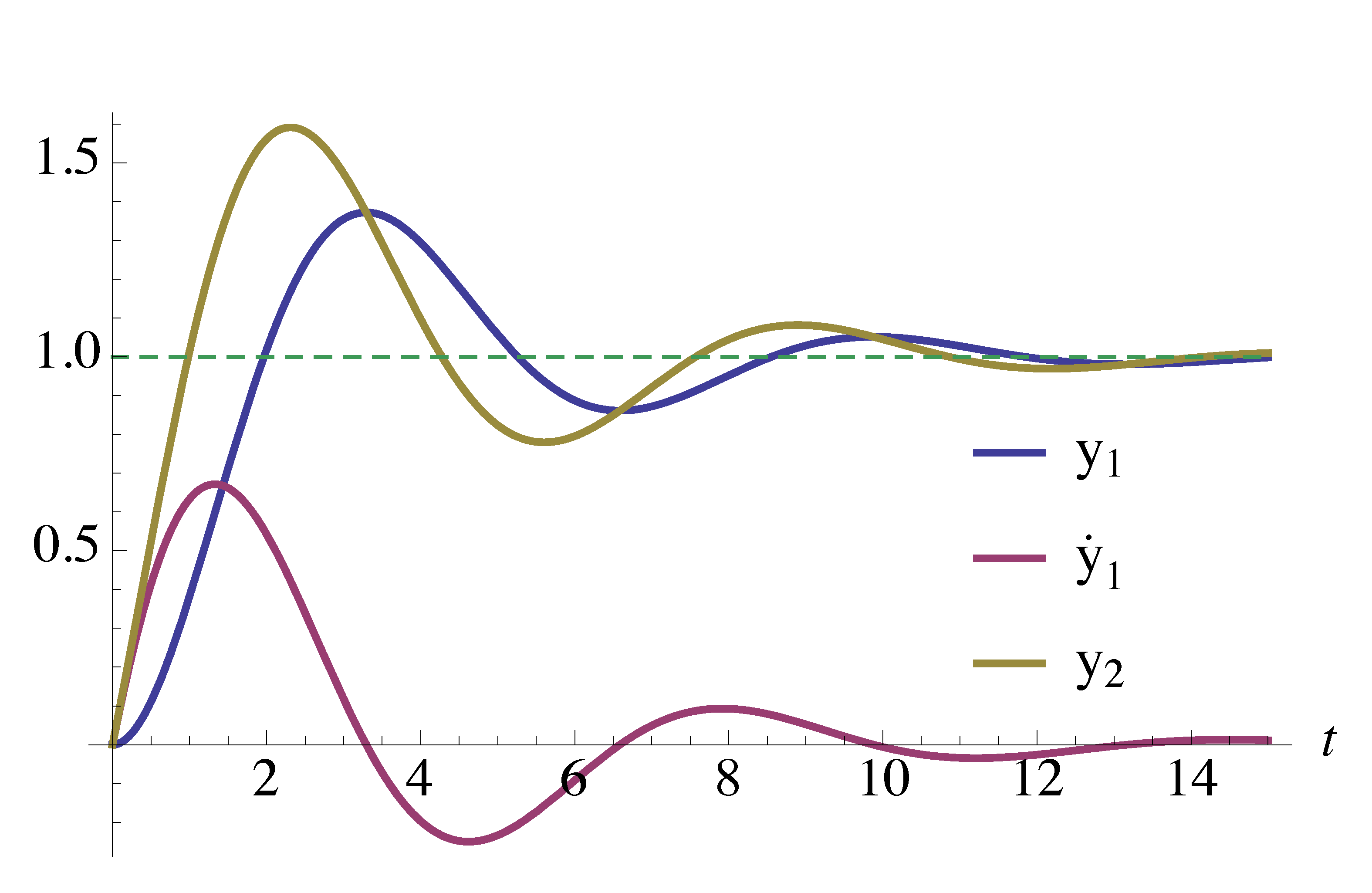
Figure 1: Effect of a LHP extra zero \(s = -a\) on step response of \(H_1(s)\)
Based on Figure 1, we noticed a LHP zero
- increased overshoot (its major effect);
- had little influence on settling time;
- and when the extra zero is far from origin, i.e., \(a \to \infty\), its effects become less significant since \(\frac{1}a \dot{y}_1(t) \to 0\).
Extra Zero on Right Half Plane
Similarly, we can consider a RHP extra zero \(s = a\) with \(a > 0\).
\begin{align*} H_1(s) = \frac{1}{s^2 + 2\zeta s + 1} \,\, \xrightarrow{\text{add zero at $s= a$}} \,\, H_2(s) &= H_1(s) - \frac{1}{a} \cdot sH_1(s), \\ \tag{2} \label{d7_eq2} y_2(t) &= y_1(t) - \frac{1}{a} \cdot \dot{y}_1(t). \end{align*}Equation \eqref{d7_eq2} says when the extra zero is on the RHP, instead of summing up the original response \(y_1(t)\) and its derivative \(\dot{y}_1(t)\), we subtract the scaled derivative term \(\frac{1}a \dot{y}_1(t)\) from the original response \(y_1(t)\).

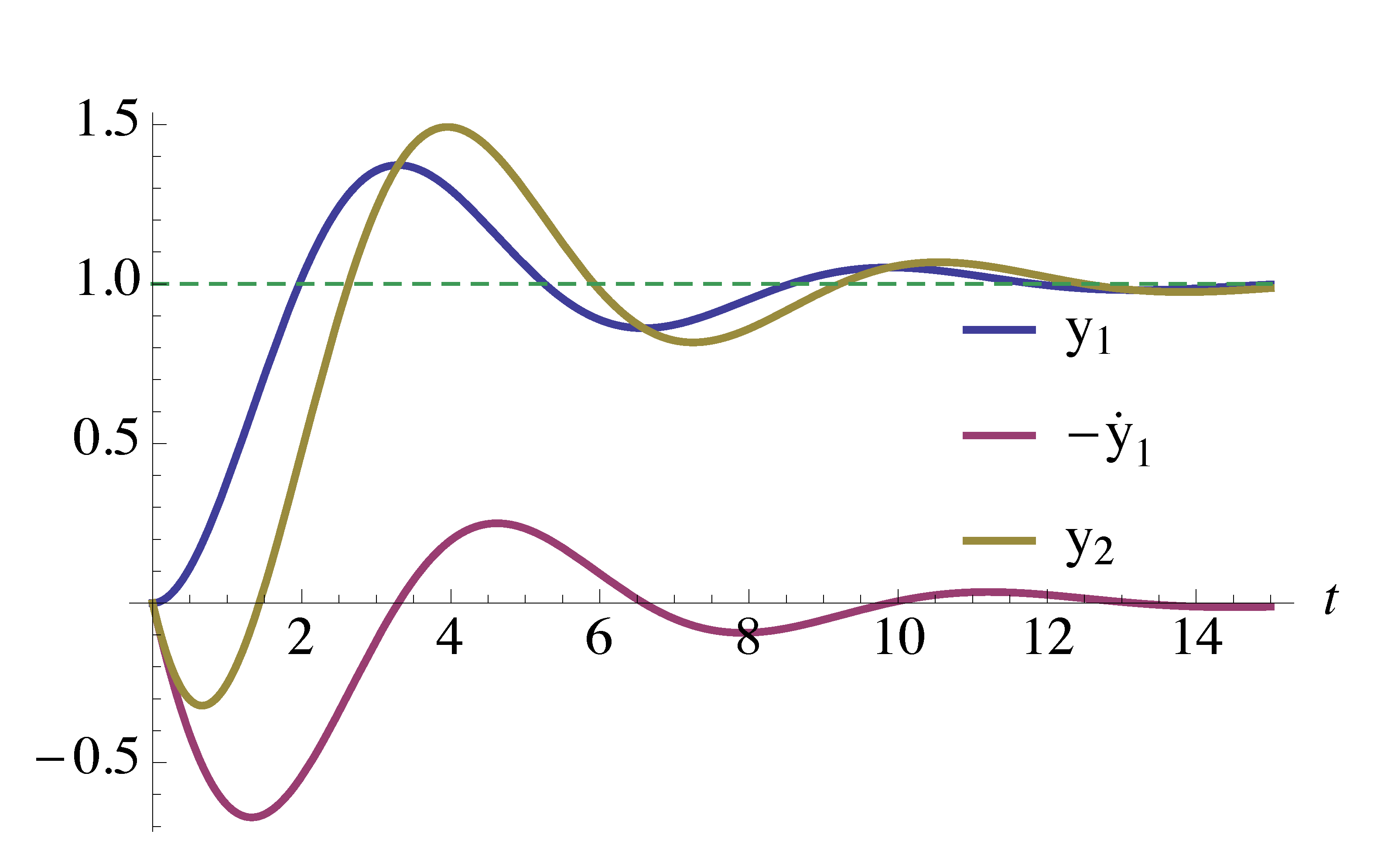
Figure 2: Effect of a RHP extra zero \(s = a\) on step response of \(H_1(s)\)
Based on Figure 2, a RHP zero
- slowed down (or delayed) the original response;
- created significant undershoot when the extra zero is close to origin, i.e., \(a\) is small enough.
Effect of Poles
Poles on Left Half Plane
A general $n$th-order system has \(n\) (complex) poles since by Fundamental theorem of algebra the polynomial equation \(p(s) = 0\) has exactly \(n\) roots in \(\CC\). Further we observe
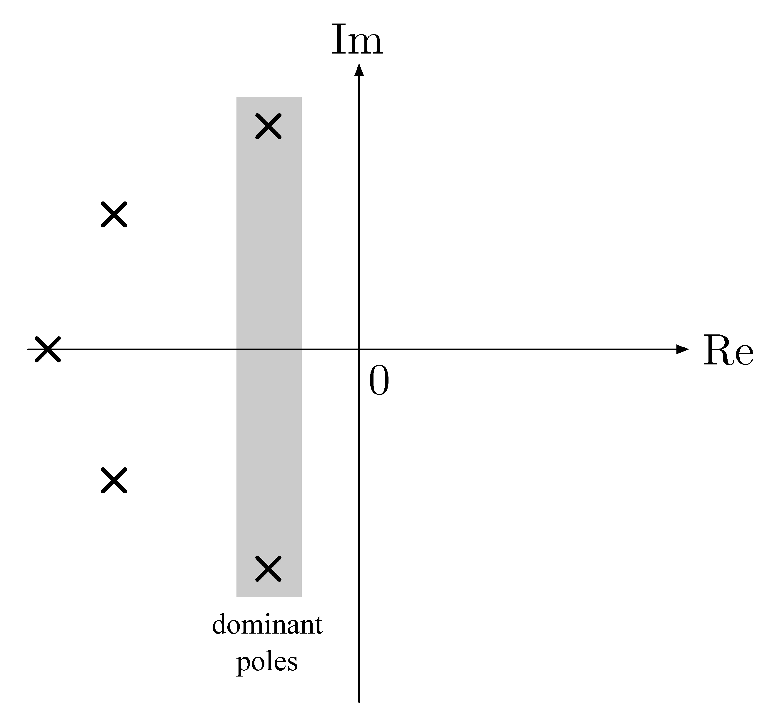
- LHP poles are not significant if their real parts are at least \(5\) times the real parts of dominant LHP poles, e.g., if dominant poles have \({\rm Re}(s) = -2\) and we have extra poles with \({\rm Re}(s) = -10\), their time-domain contributions will be \(e^{-2t}\) and \(e^{-10t}\) but \(e^{-10t} \ll e^{-2t}\) decays much faster;
the “\(5\) times” is just a convention, but we can really see the effect of poles that are closer. (cf. Lab 2)

Poles on Right Half Plane
We do not want to consider RHP poles in general since these are unstable poles.
Poles on Imaginary Axis
The boundary case is when the poles lie on the imaginary axis.
First consider the case of a pole at the origin \[H(s) = \dfrac{1}{s}.\]
Is this a stable system?
- To compute its impulse response: \(Y(s) = \dfrac{1}{s} \implies y(t) = 1(t)\), output is a unit, hence a stable output.
- To compute its step response: \(Y(s) = \dfrac{1}{s^2} \implies y(t) = t, \, t \ge 0\), output is a unit ramp, hence growing indefinitely.
Next consider the case of a pair of purely imaginary poles \[H(s) = \dfrac{\omega^2}{s^2 + \omega^2}.\]
- To compute its impulse response: \(Y(s) = \dfrac{\omega^2}{s^2+\omega^2} \implies y(t) = \omega \sin (\omega t)\), hence output is bounded but not convergent.
- To compute its step response: \(Y(s) = \dfrac{\omega^2}{s(s^2+\omega^2)} \implies y(t) = 1 - \cos(\omega t)\), again the output is bounded but not convergent.
Therefore, systems with poles on the imaginary axis are not strictly stable.
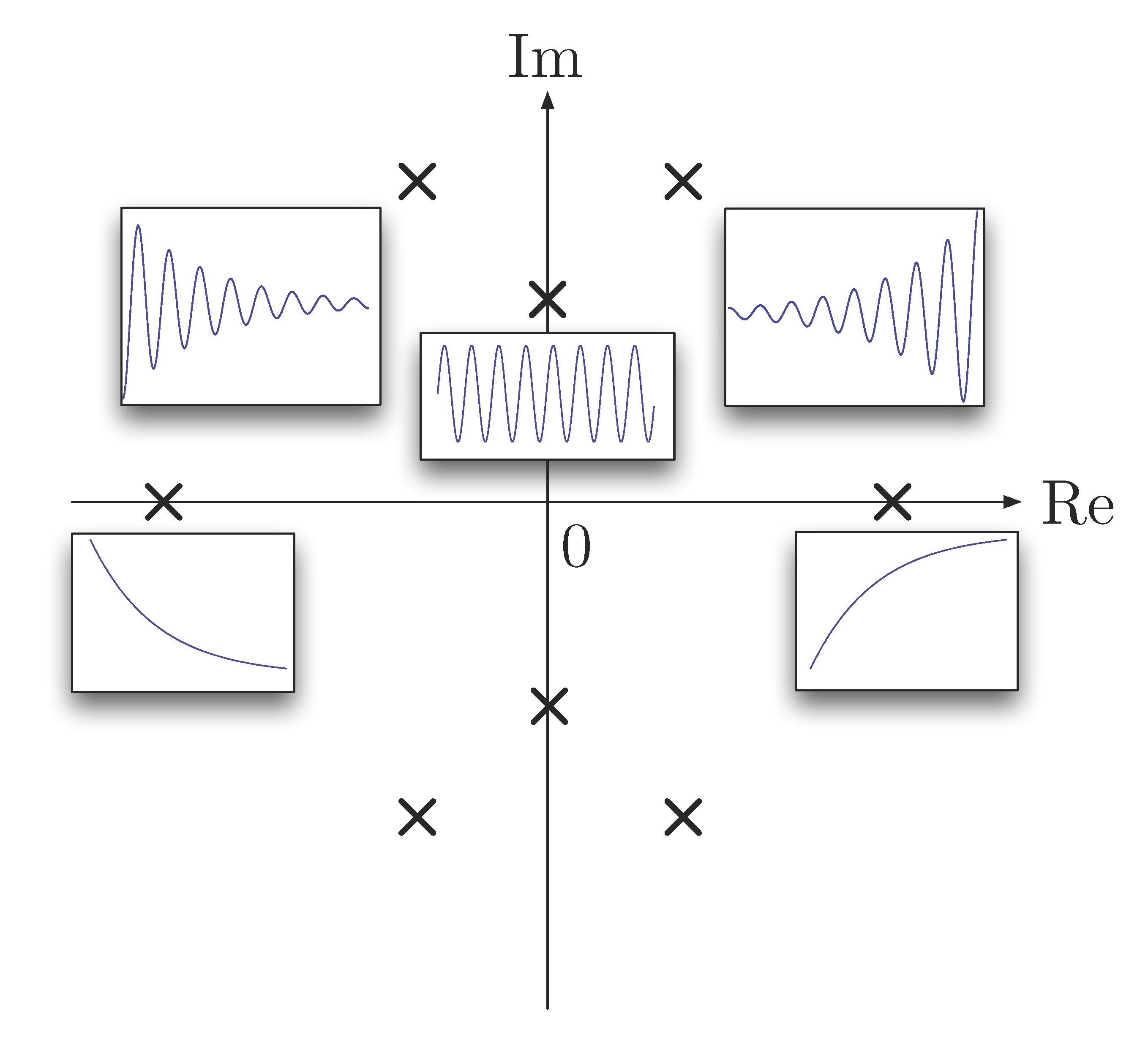
To illustrate what we have discussed so far, Figure 4 shows

Figure 4: Effect of poles on step response of \(H(s)\)
Correction: The shape of the subfigure in Figure 4 is not correct in the case of a blowing up exponential for real positive poles. The shape of this subfigure shall be a reflection with respect to $y$-axis of the figure in the case of a decaying exponential for real negative poles, not with respect to $x$-axis.
- poles in open LHP \({\rm Re}(s) < 0\), system response is stable
- poles in open RHP \({\rm Re}(s) > 0\), system response is unstable
- poles on the imaginary axis \({\rm Re}(s) = 0\), system response is not strictly stable.
Input-Output Stability
Recall the input-output set-up we used in Lecture 4,

A linear time-invariant system is said to be Bounded-Input, Bounded-Output (BIBO) stable provided either one of the following three equivalent conditions is satisfied:
- If every bounded input \(u(t)\) results in a bounded output \(y(t)\), regardless of initial conditions.
- If the impulse response \(h(t)\) is absolutely integrable, \[ \int^\infty_{-\infty}\left|h(t)\right|\d t < \infty. \]
- If all poles of the transfer function \(H(s)\) are strictly stable, i.e., all of them lie in the Open Left Half Plane.
Checking for Stability
Consider a general proper transfer function \[ H(s) = \frac{q(s)}{p(s)}, \] where \(q(s)\) and \(p(s)\) are polynomials, and \({\rm deg}(q) \le {\rm deg}(p)\).
We need to develop machinery to check system stability, i.e., whether or not all roots of \(p(s) = 0\) lie in Open Left Half Plane (OLHP). For simple polynomials, we can run stability checking via factoring them “by inspection” and find roots.
This is hard however to do for high-degree polynomials; it’s computationally intensive, and there is no closed form formula in simple operations for polynomials with degrees greater than or equal to \(5\). (Why?) Hint: See Abel-Ruffini. Often we don’t need to know the precise pole locations, we just need to know whether they are strictly stable poles, i.e., lying in the OLHP.
Question: Given an $n$th-degree polynomial \[ p(s) = s^n + a_1 s^{n-1} + a_2 s^{n-2} + \ldots + a_{n-1} s + a_n, \]
with real coefficients, check that the roots of the equation \(p(s) = 0\) are strictly stable (i.e., have negative real parts).
Terminology:
- We often say that the polynomial \(p\) is (strictly) stable if all of its roots are (strictly) stable.
- We say that \(A\) is a necessary condition for \(B\) if \[ A \text{ is false } \implies B \text{ is false}, \] or \[ B \text{ is true } \implies A \text{ is true}. \] This means even if \(A\) is true, \(B\) may still be false.
- We say that \(A\) is a sufficient condition for \(B\) if \[ A \text{ is true } \implies B \text{ is true}. \]
- Thus, \(A\) is a necessary and sufficient condition for \(B\) if \[ A \text{ is true} \iff B \text{ is true}, \] it reads \(A\) is true if and only if (iff) \(B\) is true.
Necessary condition for stability: A polynomial \(p\) is strictly stable only if all of its coefficients are strictly positive.
Proof: Suppose that \(p\) has roots at \(r_1, r_2, \cdots, r_n\) with \({\rm Re}(r_i) < 0\) for all \(i\), then
\begin{align*} p(s) = (s-r_1)(s-r_2)\cdots(s-r_n). \end{align*}Multiply this out and check that all coefficients are positive. (Why?) Hint: For complex roots, they appear in pairs. (Why?) For each pair, they belong to a factor \(s^2 - (r_i + \bar{r}_i) s + r_i \bar{r}_i\) of the polynomial \(p(s)\). This factor has real coefficients since \(r_i + \bar{r}_i = 2 {\rm Re}(r_i)\) and \(r_i \bar{r}_i = |r_i|^2\).
Routh–Hurwitz Criterion
We will now introduce a necessary and sufficient condition for stability, the Routh–Hurwitz Criterion.
Routh–Hurwitz Criterion: A Bit of History

Figure 6: James Clerk Maxwell
J.C. Maxwell, On governors, Proc. Royal Society, no. 100, 1868
… Stability of the governor is mathematically equivalent to the condition that all the possible roots, and all the possible parts of the impossible roots, of a certain equation shall be negative …
I have not been able completely to determine these conditions for equations of a higher degree than the third; but I hope that the subject will obtain the attention of mathematicians.

Figure 7: Edward John Routh, 1831–1907
In 1877, Maxwell was one of the judges for the Adams Prize, a biennial competition for best essay on a scientific topic. The topic that year was stability of motion. The prize went to Edward John Routh, who solved the problem posed by Maxwell in 1868.

Figure 8: Adolf Hurwitz, 1859–1919
In 1893, Adolf Hurwitz solved the same problem, using a different method, independently of Routh.
Routh’s Test: check whether the polynomial \[ p(s) = s^n + a_1 s^{n-1} + a_2 s^{n-2} + \cdots + a_{n-1}s + a_n \] is strictly stable.
We begin by forming the Routh array using the coefficients of \(p(s)\),
\begin{align*} \begin{matrix} s^n : & 1 & a_2 & a_4 & a_6 &\ldots \\ s^{n-1}: & a_1 & a_3 & a_5 & a_7 &\ldots \end{matrix} \end{align*}If necessary, add zeros in the second row to match lengths. Note that the very first entry is always \(1\), and also note the order in which the coefficients are filled in: from left to right, odd numbered coefficients are in the first row; even numbered coefficients are in the second.
Next, we form the third row marked by \(s^{n-2}\). The computation of coefficients in the current row is based on the coefficients in the immediate previous two rows.
\begin{align*} \begin{matrix} s^n : & 1 & a_2 & a_4 & a_6 &\ldots \\ s^{n-1}: & a_1 & a_3 & a_5 & a_7 &\ldots \\ s^{n-2}: & b_1 & b_2 & b_3 & \ldots & \end{matrix} \end{align*}where
\begin{align*} b_1 &= -\frac{1}{a_1} \det \left( \begin{matrix} 1 & a_2 \\ a_1 & a_3 \end{matrix} \right) \\ &= -\frac{1}{a_1}\left( a_3 - a_1 a_2 \right), \\ b_2 &= -\frac{1}{a_1} \det \left( \begin{matrix} 1 & a_4 \\ a_1 & a_5 \end{matrix} \right) \\ &= -\frac{1}{a_1}\left( a_5 - a_1 a_4 \right), \\ b_3 &= -\frac{1}{a_1} \det \left( \begin{matrix} 1 & a_6 \\ a_1 & a_7 \end{matrix} \right) \\ &= -\frac{1}{a_1}\left( a_7 - a_1 a_6 \right), \\ &\text{ and so on ...} \end{align*}Notice that the new row is \(1\) element shorter than the one above it.
Similar to \(s^{n-2}\), we can construct the fourth row \(s^{n-3}\) by coefficients from the second and third rows,
\begin{align*} \begin{matrix} s^n : & 1 & a_2 & a_4 & a_6 &\ldots \\ s^{n-1}: & a_1 & a_3 & a_5 & a_7 &\ldots \\ s^{n-2}: & b_1 & b_2 & b_3 & \ldots & \\ s^{n-3}: & c_1 & c_2 & \ldots & & \end{matrix} \end{align*}where
\begin{align*} c_1 &= -\frac{1}{b_1} \det \left( \begin{matrix} a_1 & a_3 \\ b_1 & b_2 \end{matrix} \right) \\ &= -\frac{1}{b_1}\left( a_1 b_2 - a_3 b_1 \right), \\ c_2 &= -\frac{1}{b_1} \det \left( \begin{matrix} a_1 & a_5 \\ b_1 & b_3 \end{matrix} \right) \\ &= -\frac{1}{b_1}\left( a_1 b_3 - a_5 b_1 \right), \\ &\text{ and so on ...} \end{align*}Eventually, we complete the array
\begin{align*} \begin{matrix} s^n : & 1 & a_2 & a_4 & a_6 & \ldots \\ s^{n-1} : & a_1 & {a_3} & {a_5} & {a_7} & \ldots \\ s^{n-2}: & b_1 & {b_2} & {b_3} &\ldots \\ s^{n-3}: & c_1 & {c_2} & \ldots \\ \vdots & \\ s^1 : & * & * \\ s^0: & * \end{matrix} \end{align*}as long as we don’t get stuck with division by zero. (More on this later.)
After the process terminates, we will have \(n+1\) entries in the first column.
The Routh–Hurwitz Criterion: Consider $n$-th degree polynomial \[ p(s) = s^n + a_1 s^{n-1} + \ldots + a_{n-1}s + a_n \] and form the Routh array:
\begin{align*} \begin{matrix} s^n : & {1} & a_2 & a_4 & a_6 & \ldots \\ s^{n-1} : & {a_1} & {a_3} & {a_5} & {a_7} & \ldots \\ s^{n-2}: & {b_1} & {b_2} & {b_3} &\ldots \\ s^{n-3}: & {c_1} & {c_2} & \ldots \\ \vdots & \\ s^1 : & * & * \\ s^0: & * \end{matrix} \end{align*}Assume that the necessary condition for stability holds, i.e., \(a_1,\ldots,a_n > 0\), then
- \(p(s)\) is stable if and only if all entries in the first column of Routh array are positive; otherwise,
- \(\# \text{(RHP poles)} = \# \text{(sign changes in first column of Routh array)}\).
Example 2: Determine the stability of polynomial \[ p(s) = s^4 + 4s^3 + s^2 + 2s + 3. \]
Solution: All coefficients strictly positive, i.e., necessary condition holds. Compute the Routh array as follows,
\begin{align*} \begin{matrix} s^4: & 1 & 1 & 3 \\ s^3: & 4 & 2 & 0 \\ s^2: & \frac{1}2 & 3 \\ s^1: & -22 & 0 \\ s^0: & 3 \end{matrix} \end{align*}Therefore \(p(s)\) is unstable. It has \(2\) RHP poles since there are \(2\) sign changes in first column of the above Routh array.
Example 3: Apply Routh–Hurwitz criterion to low-order polynomials when \(n=2,3\). Obtain shortcuts for those cases.
Solution: When \(n = 2\), consider \(p(s) = s^2 + a_1 s + a_2\). The corresponding Routh array is
\begin{align*} \begin{matrix} s^2: & 1 & a_2 \\ s^1: & a_1 & 0 \\ s^0: & b_1 & \end{matrix} \end{align*}where
\begin{align*} b_1 &= -\frac{1}{a_1}\det\left( \begin{matrix} 1 & a_2 \\ a_1 & 0 \end{matrix}\right) \\ &= a_2. \end{align*}Thus \(p(s)\) is stable if and only if \(a_1,a_2 > 0\).
Similarly, when \(n = 3\), consider \(p(s) = s^3 + a_1 s^2 + a_2 s + a_3\). The corresponding Routh array is
\begin{align*} \begin{matrix} s^3: & 1 & a_2 \\ s^2: & a_1 & a_3 \\ s^1: & b_1 & 0 \\ s^0: & c_1 & \end{matrix} \end{align*}where
\begin{align*} b_1 &= -\frac{1}{a_1}\det\left( \begin{matrix} 1 & a_2 \\ a_1 & a_3 \end{matrix}\right) \\ &= \frac{a_1a_2-a_3}{a_1}, \\ c_1 &= -\frac{1}{b_2}\det\left( \begin{matrix} a_1 & a_3 \\ b_1 & 0 \end{matrix}\right) \\ &= a_3. \end{align*}Thus \(p(s)\) is stable if and only if \(a_1,a_2,a_3 > 0\) and \(a_1 a_2 > a_3\).
Upshot: From the above two examples, we observe
- A 2nd-degree polynomial \(p(s) = s^2 + a_1 s + a_2\) is stable if and only if \(a_1 > 0\) and \(a_2 > 0\).
- A 3rd-degree polynomial \(p(s) = s^3 + a_1 s^2 + a_2 s + a_3\) is stable if and only if \(a_1,a_2,a_3 > 0\) and \(a_1a_2 > a_3\).
These conditions were already obtained by Maxwell in 1868. In both cases, the computations were purely symbolic. This can make a lot of difference in design as opposed to analysis.
Routh–Hurwitz Criterion as a Design Tool
We can use the Routh test to determine parameter ranges for stability.
Example 4: Consider the unity feedback configuration in Figure 9,

Figure 9: Example 4, Unity Feedback
determine the range of values the scalar gain \(K\) can take, for which the closed-loop system is stable.
Note that the plant itself is unstable since the denominator has a negative coefficient and a zero coefficient.
Solution: Let’s first write down the transfer function from reference \(R\) to output \(Y\),
\begin{align*} \frac{Y}{R} &= \frac{\text{forward gain}}{1 + \text{loop gain}} \\ &= \frac{K \cdot \frac{s+1}{s^3 +2s^2 -s}}{1 + K\cdot\frac{s+1}{s^3 + 2s^2 - s} } \\ &= \frac{K (s+1)}{s^3 + 2s^2 - s + K(s+1)} \\ &= \frac{Ks+K}{s^3 + 2s^2 + (K-1)s + K}. \end{align*}Now we need to test stability of \(p(s) = s^3 + 2s^2 + (K-1)s + K\) using the Routh test.
Form the Routh array:
\begin{align*} \begin{matrix} s^3 : & 1 & K-1 \\ s^2 : & 2 & K \\ s^1 : & \frac{K}2 - 1 & 0 \\ s^0 : & K \end{matrix} \end{align*}For \(p\) to be stable, all entries in the first column must be positive, i.e., \(\frac{K}2 - 1> 0\) and \(K>0\). The necessary condition requires \(K > 1\), but now we actually know that we must have \(K > 2\) for stability.
Comments on the Routh Test:
- The result \(\#\text{(RHP roots)}\) is not affected if we multiply or divide any row of the Routh array by an arbitrary positive number.
- If we get a zero element in the first column, we can’t continue. In that case, we can replace the \(0\) by a small number \(\varepsilon\) and apply Routh test to \(\varepsilon\). When we are done with the array, take the limit as \(\varepsilon \to 0\). More on this can be found in Example 3.33 in FPE.
- For an entire row of zeros, the procedure is a more complicated (see Example 3.34 in FPE). We shall not worry about this too much.