CS440/ECE448 Spring 2022 Assignment 2: Perceptron and Neural Nets Due date: Monday Feb 14th, 11:59pm

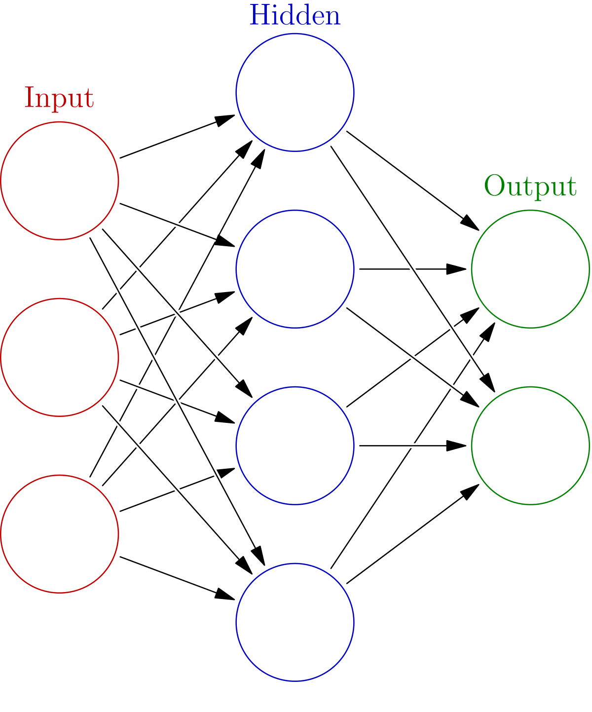
image from Wikipedia

The goal of this assignment is to employ a single perceptron and its nonlinear extension (known as neural networks) to detect whether or not images contain animals.

In the first part, you will create a single perceptron, while in the second part, you will improve it by using its non-linear extension in the form of shallow neural network.

For the part 1 (perceptron) : You may use NumPy to program your solution. Aside from that library, no other outside non-standard libraries can be used.

For part 2 (neural nets) : You will be using the PyTorch and NumPy libraries to implement neural net. The PyTorch library will do most of the heavy lifting for you, but it is still up to you to implement the right high-level instructions to train the model.

Contents

• Dataset
• Part 1: Perceptron
• Part 2: Neural Networks
• Provided Code Skeleton
• Deliverables
• Extra Credits

Dataset

The dataset consists of 10000 32x32 colored images (a subset of the CIFAR-10 dataset, provided by Alex Krizhevsky), split for you into 7500 training examples (of which 2999 are negative and 4501 are positive) and 2500 development examples.

The data set is included within the coding template available here: mp2-template.zip . When you uncompress this you'll find a binary object that our reader code will unpack for you.

Part 1: Perceptron

The perceptron model is a linear function that tries to separate data into two or more classes. It does this by learning a set of weight coefficients \(w_i\) and then adding a bias \(b\). Suppose you have features \(x_1,\dots,x_n\) then this can be expressed in the following fashion: \[ f_{w,b} (x) = \sum_{i=1}^n w_i x_i + b \] You will use the perceptron learning algorithm to find good weight parameters \(w_i\) and \(b\) such that \(\mathrm{sign}(f_{w,b}(x)) > 0\) when there is an animal in the image and \(\mathrm{sign}(f_{w,b}(x)) \leq 0\) when there is a no animal in the image.

Your function classifyPerceptron() will take as input the training data, training labels, development data, learning rate, and maximum number of iterations. It should return a list of labels for the development data. Do not hardcode values for tuning parameters inside your classifier functions, because the autograder tests pass in specific values for these parameters.

Training and Development

Please see the textbook and lecture notes for the perceptron algorithm. You will be using a single classical perceptron whose output is either positive or negative (i.e. sign/step activation function).

You may use NumPy to program your solution. Aside from that library, no other outside non-standard libraries can be used (PyTorch is NOT allowed for part 1).

The autograder will supply the set of test images as one giant numpy array. The development data is in the same format. So your code must read the dimensions from the input numpy array.

In the dataset, each image is 32x32 and has three (RGB) color channels, yielding 32*32*3 = 3072 features. However, be aware that synthetic tests in the autograder may have different dimensions. So do not hardcode the dimensions.

• Training: To train the perceptron you are going to need to implement the perceptron learning algorithm on the training set. Each pixel of the image is a feature in this case. Be sure to initialize weights and biases to zero.
  Note: To get full points on the autograder, use a constant learning rate (no decay) and do not shuffle the training data.

   

• Development: After you have trained your perceptron classifier, you will have your model decide whether or not each image in the development set contains animals. In order to do this take the sign of the function \(f_{w,b}(x)\). If it is negative or zero then classify as \(0\). If it is positive then classify as \(1\).

Use only the training set to learn the weights.

If designed correctly, the perceptron model should give you accuracy of around 0.78 to 0.80 on development set.

Some comments on Using Numpy

For this part, you are allowed to use only the NumPy. Note that it is much easier to write fast code by using numpy operations. Your data is provided as a numpy array. Use numpy operations as much as possible, until right at the end when you choose a label for each image and produce the output list of labels.

NumPy Tips:

• Running computations on arrays tend to be faster when run using NumPy arrays. If you are having issues with timing out, then consider using a NumPy implementation
• Linear algebra operators (dot product, vector norm, matrix multiplication) are immensely simplified when using NumPy. Consider looking up methods to perform some of these operations if they are needed in your solution.
• NumPy Broadcasting may make your life easier for this assignment.

Part 2: Classical Neural Network

The basic neural network model consists of a sequence of hidden layers sandwiched by an input and output layer. Input is fed into it from the input layer and the data is passed through the hidden layers and out to the output layer. Induced by every neural network is a function \(F_{W}\) which is given by propagating the data through the layers.

To make things more precise, in lecture you learned of a function \( f_{w}(x) = \sum_{i=1}^n w_i x_i + b\). In this assignment, given weight matrices \(W_1,W_2\) with \(W_1 \in \mathbb{R}^{h \times d}\), \(W_2 \in \mathbb{R}^{h \times 2}\) and bias vectors \(b_1 \in \mathbb{R}^{h}\) and \(b_2 \in \mathbb{R}^{2}\), you will learn a function \( F_{W} \) defined as \[ F_{W} (x) = W_2\sigma(W_1 x + b_1) + b_2 \] where \(\sigma\) is your activation function. In part 2, you should use either of the sigmoid or ReLU activation functions. You will use 32 hidden units (\(h=32\)) and 3072 input units, one for each channel of each pixel in an image (\(d=(32)^2(3) = 3072\)).

Training and Development

• Training: To train the neural network you are going to need to minimize the empirical risk \(\mathcal{R}(W)\) which is defined as the mean loss determined by some loss function. For this assignment you can use cross entropy for that loss function. In the case of binary classification, the empirical risk is given by \[ \mathcal{R}(W) = \frac{1}{n}\sum_{i=1}^n y_i \log \hat y_i + (1-y_i) \log (1 - \hat y_i) . \] where \(y_i\) are the labels and \(\hat y_i \) are determined by \(\hat y_i = \sigma(F_{W}(x_i))\) where \(\sigma(x) = \frac{1}{1+e^{-x}}\) is the sigmoid function. For this assignment, you won't have to implement these functions yourself; you can use the built-in PyTorch functions.

  Notice that because PyTorch's CrossEntropyLoss incorporates a sigmoid function, you do not need to explicitly include an activation function in the last layer of your network.

• Development: After you have trained your neural network model, you will have your model decide whether or not images in the development set contain animals in them. This is done by evaluating your network \(F_{W}\) on each example in the development set, and then taking the index of the maximum of the two outputs (argmax).
• Data Standardization: Convergence speed and accuracies can be improved greatly by simply centralizing your input data by subtracting the sample mean and dividing by the sample standard deviation. More precisely, you can alter your data matrix \(X\) by simply setting \(X:=(X-\mu)/\sigma\).

With the aforementioned model design and tips, you should expect around 0.84 dev-set accuracy.

Some things to look for:

1. The autograder runs the training process for 500 batches (max_iter=500). This is done so that we have a consistent training process for each evaluation and comparison with benchmarks/threshold accuracies.
2. You still have one thing in your full control, however—the learning rate. In case you are confident about a model you implemented but are not able to pass the accuracy thresholds on gradescope, you can try increasing the learning rate. It is certainly possible that your model could do better with more training. Be mindful, however, that using a very high learning rate might deteriorate performance as well since the model may begin to oscillate around the optima.

Provided Code Skeleton

We have provided a template (zip) that contains all the code and the data to get you started on your MP, which means you will only have to implement the Numpy perceptron in perceptron.py, and PyTorch neural net in neuralnet.py. Please make use of mp2_part1.py and mp2_part2.py to run the models you've implemented. These would also provide you a feedback on the performance of your models to help you rectify any issues before you submit the final version to the gradescope autograder.

• reader.py - This file is responsible for reading in the data set. It creates a giant NumPy array of feature vectors corresponding to each image. Note that part1 and patr2 share the same data set.
• mp2_part1.py - This is the main file that starts the program of part 1, and computes the accuracy, precision, recall, and F1-score using your implementation of part1.
• mp2_part2.py - This is the main file that starts the program, and computes the accuracy, precision, recall, and F1-score using your implementation of part2.
• perceptron.py is file where you will be doing all of your work for part1.
• neuralnet.py is file where you will be doing all of your work for part 2. You are given a NeuralNet class which implements a torch.nn.module. This class consists of __init__(), forward(), and step() functions. (Beyond the important details below, more on what each of these methods in the NeuralNet class should do is given in the skeleton code.)
  • __init__() is where you will need to construct the network architecture. There are multiple ways to do this.
    • One way is to use the Linear and Sequential objects. Keep in mind that Linear uses a Kaiming He uniform initialization to initialize the weight matrices and sets the bias terms to all zeros.
    • Another way you could do things is by explicitly defining weight matrices W1, W2, ... and bias terms b1, b2, ... by defining them as Tensors. This approach is more hands on and will allow you to choose your own initialization. For this assignment, however, Kaiming He uniform initialization should suffice and should be a good choice.
    Additionally, you can initialize an optimizer object in this function to use to optimize your network in the step() function.
  • get_parameters() should do what its name suggests--namely, return a list of parameters used in the model. 
  • set_parameters() should do what its name suggests--namely, set the parameters of the model based on those input to this method. For consistency's sake, the order of the parameters should be the same as those returned in get_parameters(). 
  • forward() should perform a forward pass through your network. This means it should explicitly evaluate \(F_{W}(x)\) . This can be done by simply calling your Sequential object defined in __init__() or (if you opted to define tensors explicitly) by multiplying through the weight matrices with your data.
  • step() should perform one iteration of training. This means it should perform one gradient update through one batch of training data (not the entire set of training data). You can do this by either calling loss_fn(yhat,y).backward() then updating the weights directly yourself, or you can use an optimizer object that you may have initialized in __init__() to help you update the network. Be sure to call zero_grad() on your optimizer in order to clear the gradient buffer. When you return the loss_value from this function, make sure you return loss_value.item() (which works if it is just a single number) or loss_value.detach().cpu().numpy() (which separates the loss value from the computations that led up to it, moves it to the CPU—important if you decide to work locally on a GPU, bearing in mind that Gradescope won't be configured with a GPU—and then converts it to a NumPy array). This allows proper garbage collection to take place (lest your program possibly exceed the memory limits fixed on Gradescope).
  • fit() takes as input the training data, training labels, development set, and the maximum number of iterations. The training data provided is the output from reader.py. The training labels is a Tensor consisting of labels corresponding to each image in the training data. The development set is the Tensor of images that you are going to test your implementation on. The maximium number of iterations is the number you specified with --max_iter (it is 500 by default). fit() outputs the predicted labels. It should construct a NeuralNet object, and iteratively call the neural net's step() to train the network. This should be done by feeding in batches of data determined by batch size. You will use a batch size of 100 for this assignment. max_iter is the number of batches (not the number of epochs!) in your training process.
• mp2_data is the file of data set. See reader.py, mp2_part1.py and mp2_part2.py for how to load and process the data.

The only files you will need to modify are perceptron.py and neuralnet.py.

To learn more about how to run the MP, run python3 mp2_part1.py -h and python3 mp2_part2.py -h in your terminal.

You should definitely use the PyTorch documentation, linked multiple times on this page, to help you with implementation details. You can also use this PyTorch Tutorial as a reference to help you with your implementation. There are also other guides out there such as this one.

Deliverables

This MP will be submitted via Gradescope; please upload both perceptron.py (for part 1) and neuralnet.py (for part 2).

Please do not zip these two files together, but rather upload them separately. Please refer to this guide if you need help.

Extra credit: CIFAR-100 superclasses

For an extra 10% worth of the points on this MP, your task will be to pick any two superclasses from the CIFAR-100 dataset (described in the same place as CIFAR-10) and rework your neural net from part 2, if necessary, to distinguish between those two superclasses. A superclass contains 2500 training images and 500 testing images, so between two superclasses you will be working with 3/5 the amount of data in total (6000 total images here versus 10000 total in the main MP).

To begin working on the extra credit, we recommend that you make a copy of the entire directory containing your solution to the second part of the main MP. Then replace the data directory and the file reader.py, and modify your file neuralnet.py, as described in the next two paragraphs.

• Replace CIFAR-10 with CIFAR-100, and download the new reader

You can download the CIFAR-100 data here and extract it to the same place where you've placed the data for the main MP. A custom reader for it is provided here; to use it with the CIFAR-100 data, you should rename this to reader.py and replace the existing file of that name in your working directory.

• Modify neuralnet.py in order to choose the two CIFAR-100 classes you want to classify

Define two global variables class1 and class2 at the top level of the file neuralnet.py (that is, outside of the NeuralNet class). Set the values of these variables to integers, in order to choose the two classes that you want to classify for extra credit. The order of the superclasses listed on the CIFAR description page hints at the index for each superclass; for example, "aquatic mammals" is 0 and "vehicles 2" is 19.

• Now that you have the new classification task, the first thing you should do is to try running the same code that you used in part 2 of the regular MP, to re-train your neural net on these new data, then test it to see how well it performs. This can be your baseline; your goal for extra credit will be to find new algorithms that give you better accuracy. Your new algorithm can be anything you like (a network with more layers, or with more nodes per hidden layer, or a convolutional neural network, or any other algorithm of your choice). Note that your revised neural net must still have fewer than 500,000 total parameters.

The points for the extra credit are distributed as follows:

• 4 points will be granted automatically for a submission attaining an accuracy above a certain minimum threshold for the two superclasses you chose. (This threshold differs depending on your choice of superclasses to distinguish; it was determined based on the reference implementation of the main MP.)
• 3 points will be granted automatically for a submission attaining an accuracy above a certain medium threshold for the two superclasses you chose.
• 3 points will be granted automatically for a submission attaining an accuracy above a certain maximum threshold for the two superclasses you chose.