Note: This is an individual project; you can NOT work collaboratively to generate the solutions.
Due Date: 11:59pm on Wednesday, Apr. 8, 2020
Overview
The goal of this project is to familiarize yourself high dynamic range (HDR) imaging, image based lighting (IBL), and their applications. By the end of this project, you will be able to create HDR images from sequences of low dynamic range (LDR) images and also learn how to composite 3D models seamlessly into photographs using image-based lighting techniques. HDR tonemapping can also be investigated as bells and whistles.
HDR photography is the method of capturing photographs containing a greater dynamic range than what normal photographs contain (i.e. they store pixel values outside of the standard LDR range of 0-255 and contain higher precision). Most methods for creating HDR images involve the process of merging multiple LDR images at varying exposures, which is what you will do in this project.
HDR images are widely used by graphics and visual effects artists for a variety of applications, such as contrast enhancement, hyper-realistic art, post-process intensity adjustments, and image-based lighting. We will focus on their use in image-based lighting, specifically relighting virtual objects. One way to relight an object is to capture an 360 degree panoramic (omnidirectional) HDR photograph of a scene, which provides lighting information from all angles incident to the camera (hence the term image-based lighting). Capturing such an image is difficult with standard cameras, because it requires both panoramic image stitching (which you will see in project 5) and LDR to HDR conversion. An easier alternative is to capture an HDR photograph of a spherical mirror, which provides the same omni-directional lighting information (up to some physical limitations dependent on sphere size and camera resolution). We will take the spherical mirror approach, inspired primarily by Debevec's paper. With this panoramic HDR image, we can then relight 3D models and composite them seamlessly into photographs. This is a very quick method for inserting computer graphics models seamlessly into photographs and videos; much faster and more accurate than manually "photoshopping" objects into the photo.
Recovering HDR Radiance Maps (50 pts)
To the right are three pictures taken with different exposure times (1/24s, 1/60s, 1/120s) of a spherical mirror in my office. The rightmost image shows the HDR result (tonemapped for display). In this part of the project, you'll be creating your own HDR images. First, you need to collect the data.
What you need:
Spherical mirror (see Piazza post)
Camera with exposure time control. This is available on all DSLRs and most point-and-shoots, and even possible with most mobile devices using the right app; e.g. ProCamera on iOS, Camera FV-5 Lite on Android (this even has auto exposure bracketing, AEB). Automatic exposure bracketing is helpful but not really needed.
Tripod / rigid surface to hold camera / very stead hand (not recommended)
Data collection (10 points)
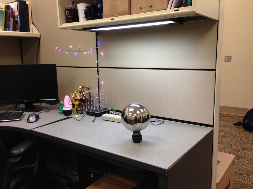
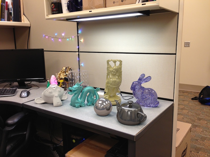
Find a good scene to photograph. The scene should have a flat surface to place your spherical mirror on (see my example below). Either indoors or outdoors will work.
Find a fixed, rigid spot to place your camera. A tripod is best, but you can get away with less. I used the back of a chair to steady my phone when taking my images.
Place your spherical mirror on a flat surface, and make sure it doesn't roll by placing a cloth/bottle cap/etc under it. Make sure the sphere is not too far away from the camera -- it should occupy at least a 256x256 block of pixels.
Photograph the spherical mirror using at least three different exposure times. Make sure the camera does not move too much (slight variations are OK, but the viewpoint should generally be fixed). For best results, your exposure times should be at least 4 times longer and 4 times shorter (±2 stops) than your mid-level exposure (e.g. if your mid-level exposure time is 1/40s, then you should have at least exposure timess of 1/10s and 1/160s; the greater the range the better). Make sure to record the exposure times.
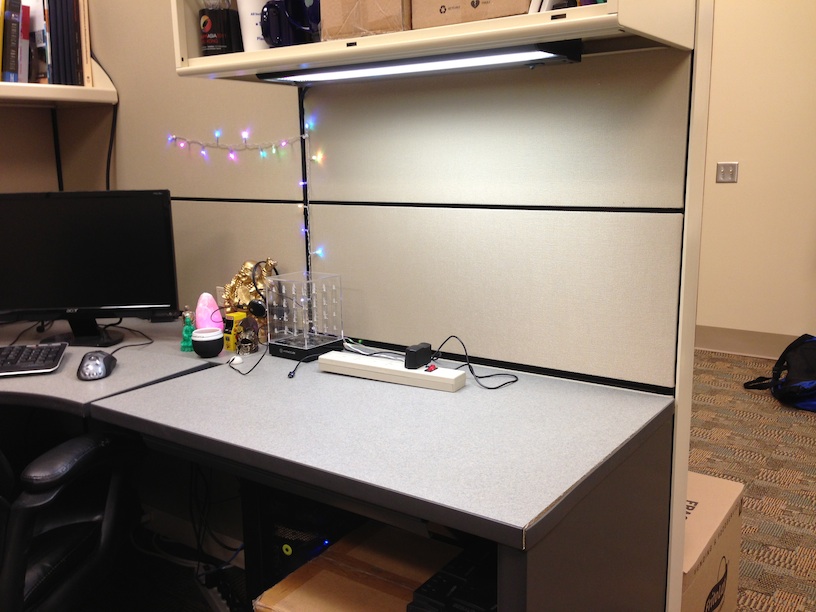
Remove the mirror from the scene, and from the same viewpoint as the other photographs, take another picture of the scene at a normal exposure level (most pixels are neither over- or under-exposed). This will be the image that you will use for object insertion/compositing (the "background" image).
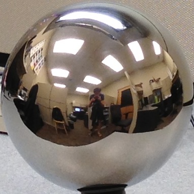
After you copy all of the images from your camera/phone to your computer, load the spherical mirror images (from step 4) into your favorite image editor and crop them down to contain only the sphere (see example below).
Small alignment errors may occur (due to camera motion or cropping). One way to fix these is through various alignment procedures, but for this project, we won't worry about these errors. If there are substantial differences in camera position/rotation among the set of images, re-take the photographs.
From left to right: one of my sphere pictures (step 4), cropped sphere (step 6), empty scene (step 5)
Naive LDR merging (10 points)
After collecting data, load the cropped images, and resize them to all be square and the same dimensions (e.g. cv2.resize(ldr,(N,N)) N is the new size). Either find the exposure times using the EXIF data (usually accessible in the image properties), or refer to your recorded exposure times. To put the images in the same intensity domain, divide each by its exposure time (e.g. ldr1_scaled = ldr1 / exposure_time1). After this conversion, all pixels will be scaled to their approximate value if they had been exposed for 1s.
The easiest way to convert your scaled LDR images to an HDR is simply to average them. Create one of these for comparison to your later results.
To save the HDR image, use given write_hdr_image function. To visualize HDR image, use given display_hdr_image function.
LDR merging without under- and over-exposed regions (10 points)
The naive method has an obvious limitation: if any pixels are under- or over-exposed, the result will contain clipped (and thus incorrect) information. A simple fix is to find these regions (e.g. a pixel might be considered over exposed if its value is less than 0.02 or greater than 0.98, assuming [0,1] images), and exclude them from the averaging process. Another way to think about this is that the naive method is extended using a weighted averaging procedure, where weights are 0 if the pixel is over/under-exposed, and 1 otherwise. Note that with this method, it might be the case that for a given pixel it is never properly exposed (i.e. always either above or below the threshold in each exposure).
There are perhaps better methods that achieve similar results but don't require a binary weighting. For example, we could create a weighting function that is small if the input (pixel value) is small or large, and large otherwise, and use this to produce an HDR image. In python, such a function can be created with: w = lambda z: float(128-abs(z-128)) assuming pixel values range in [0,255].
LDR merging and response function estimation (15 points)
Nearly all cameras apply a non-linear function to recorded raw pixel values in order to better simulate human vision. In other words, the light incoming to the camera (radiance) is recorded by the sensor, and then mapped to a new value by this function. This function is called the film response function, and in order to convert pixel values to true radiance values, we need to estimate this response function. Typically the response function is hard to estimate, but since we have multiple observations at each pixel at different exposures, we can do a reasonable job up to a missing constant.
The method we will use to estimate the response function is outlined in this paper. Given pixel values Z at varying exposure times t, the goal is to solve for g(Z) = ln(R*t) = ln(R)+ln(t). This boils down to solving for R (irradiance) since all other variables are known. By these definitions, g is the inverse, log response function. The paper provides code to solve for g given a set of pixels at varying exposures (we also provide gsolve function in our utils folder). Use this code to estimate g for each image channel (r/g/b). Then, recover the HDR image using equation 6 in the paper.
Some hints on using gsolve:
When providing input to gsolve, don't use all available pixels, otherwise you will likely run out of memory / have very slow run times. To overcome, just randomly sample a set of pixels (100 or so can suffice), but make sure all pixel locations are the same for each exposure.
The weighting function w should be implemented using Eq. 4 from the paper (this is the same function that can be used for the previous LDR merging method, i.e. w = lambda z: float(128-abs(z-128)).
Try different lambda values for recovering g. Try lambda=1 initially, then solve for g and plot it. It should be smooth and continuously increasing. If lambda is too small, g will be bumpy.
Refer to Eq. 6 in the paper for using g and combining all of your exposures into a final image. Note that this produces log radiance values, so make sure to exponentiate the result and save absolute radiance.
Panoramic transformations (10 points)
Now that we have an HDR image of the spherical mirror, we'd like to use it for relighting (i.e. image-based lighting). However, many programs don't accept the "mirror ball" format, so we need to convert it to a different 360 degree, panoramic format (there is a nice overview of many of these formats here). Most rendering software accepts this format, including Blender's Cycles renderer, which is what we'll use in the next part of the project.
To perform the transformation, we need to figure out the mapping between the mirrored sphere domain and the equirectangular domain. We can calculate the normals of the sphere (N) and assume the viewing direction (V) is constant. We then calculate reflection vectors with R = V - 2 * dot(V,N) * N, which is the direction that light is incoming from the world to the camera after bouncing off the sphere. The reflection vectors can then be converted to spherical coordinates by providing the latitude and longitude (phi and theta) of the given pixel (fixing the distance to the origin, r, to be 1). Note that this assumes an orthographic camera (which is a close approximation as long as the sphere isn't too close to the camera). The view vector is assumed to be at (0,0,-1).
Next, the equirectangular domain can be created by making an image in which the rows correspond to theta and columns correspond to phi in spherical coordinates. For this we have a function in the starter code called get_equirectangular_image() (You can find the function under utils in hdr_helpers.py). The function takes reflection vectors and the HDR image produced in the Naive implementation as input and returns the equirectangular image as output.
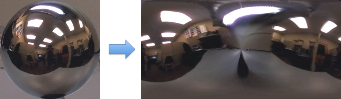
Note that by choosing 360 as EH and 720 as EW, we are making every pixel in equirectangular image to correspond to area occupied by 0.5 degree x 0.5 degree in spherical coordinate. Now that you have the phi/theta for both the mirror ball image and the equirectangular domain, use scipy's scipy.interpolate.griddata function to perform the transformation. Below is an example transformation.
Rendering synthetic objects into photographs (30 pts)
Next, we will use our equirectangular HDR image as an image-based light, and insert 3D objects into the scene. This consists of 3 main parts: modeling the scene, rendering, and compositing. Specific instructions follow below; if interested, see additional details in Debevec's paper.
Begin by downloading/installing Blender here. Note that this part of tutorial assumes that you are using blender version 2.79. If you want to use newest blender 2.8 or above, please refer to this page or this demo for step by step reference. In the course materials package below, locate the blend file under samples directory and open it. This is the blend file I used to create the result at the top of the page. The instructions below assume you will modify this file to create your own composite result, but feel free to create your own blend file from scratch if you are comfortable with Blender.
Modeling the scene
To insert objects, we must have some idea of the geometry and surface properties of the scene, as well as the lighting information that we captured in previous stages. In this step, you will manually create rough scene geometry/materials using Blender.
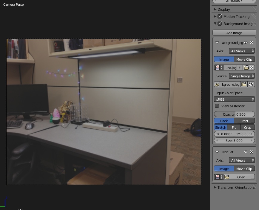
With the sample blend file open, add your background image to the scene. In the 3D view window near the bottom right, locate "Background Images". Make sure this is checked, and click "Add image", then click "Open" and locate your background image from step 4 of data collection. Make sure your view is from the camera's perspective by pressing View->Camera; you should see your image in view.
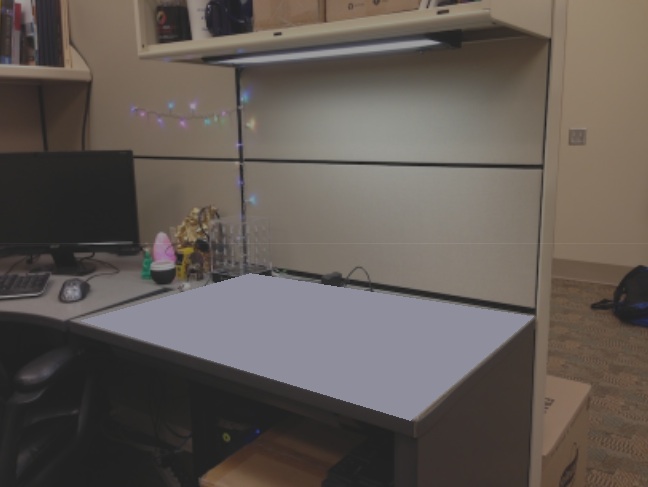
Next, model the "local scene." That is, add simple geometry (usually planes suffice) to recreate the geometry in the scene near where you'd like to insert objects. For best results, this should be close to where you placed the spherical mirror. Feel free to use the sample scene provided and move the vertices of the plane to match the surface you'd like to recreate (ignore the inserted bunny/teapot/etc for now). Once you're happy with the placement, add materials to the local scene: select a piece of local scene geometry, go to Properties->Materials, add a Diffuse BSDF material, and change the "Color" to roughly match the color from the photograph.
Then, add your HDR image (the equirectangular map made above) to the scene. First, use notebook to save the HDR panorama: write_hdr_image(eq_image, 'equirectangular.hdr'). In the Properties->World tab, make sure Surface="Background" and Color="Environment Texture". Locate your saved HDR image in the filename field below "Environment Texture".
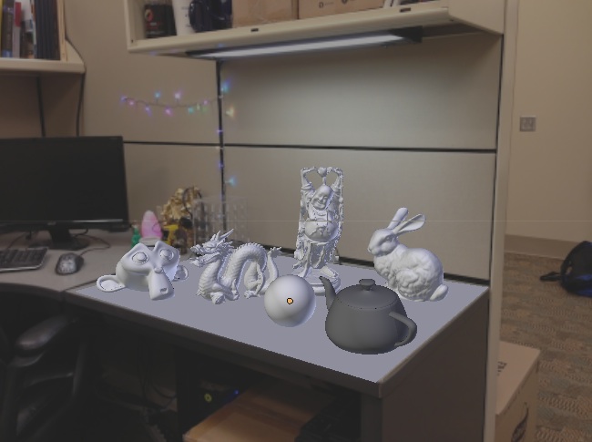
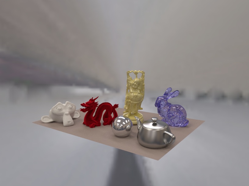
Finally, insert synthetic objects into the scene. Feel free to use the standard models that I've included in the sample blend file, or find your own (e.g. Turbosquid, Google 3D Warehouse, DModelz, etc). Add interesting materials to your inserted objects as well. Once finished, your scene should now look something like the right image below.
Blender scene after: loading background image, modeling local scene, inserting objects
Rendering
We can now render the scene to see a preview of what the inserted objects will look like. Make sure "Cycles Render" is selected at the top of Blender's interface, and then render the scene (F12). Your rendering might be too bright/dark, which is caused because we don't know the absolute scale of the lighting, so this must be set manually. To fix, adjust the light intensity (Properties->World tab, adjust "Strength" setting under "Color" accordingly). Once you're happy with the brightness, save the rendered result to disk.
My rendered scene is down below; as you can tell, this is not quite the final result. To seamlessly insert the objects, we need to follow the compositing procedure outlined by Debevec (Section 6 of the paper). This requires rendering the scene twice (both with and without the inserted objects), and creating an inserted object mask.
Next, we'll render the "empty" scene (without inserted objects). Create a copy of your blender scene and name it something like ibl-empty.blend. Open up the copy, and delete all of the inserted objects (but keep the local scene geometry). Render this scene and save the result.
Finally, we need to create an object mask. The mask should be 0 where no inserted objects exist, and greater than 0 otherwise. First, create another duplicate of your scene and open it up (e.g. ibl-mask.blend). We can create the mask quickly using Blender by manipulating object materials and rendering properties:
In the top panel, make sure it says "Blender Render" (if it says something else, e.g. Cycles Render, change it to Blender Render)
Select an object (right click on it)
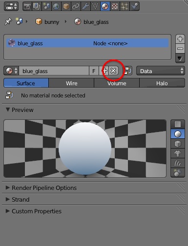
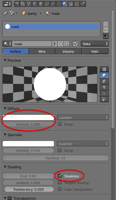
Go to the materials panel (Properties->Materials; looks like a black/red circle)
Remove the Material by pressing the 'x' (to the left of "Data")
Click "New" to add a new material
In the new material properties, under "Diffuse", change Intensity=1 and the RGB color = (1,1,1)
Under "Shading", check the "Shadeless" box
Repeat for all inserted objects
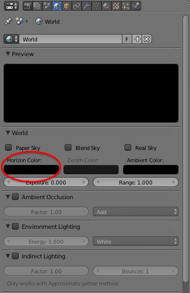
In Properties->World, set the Horizon RGB color = (0,0,0)
Render the scene and save your mask as a PNG (or some lossless format)
Visuals for steps 3-9 above.
After these steps, you should have the following three rendered images:
Rendered image with objects, rendering without objects, object mask
To simplify this process, we have created a script ibl_script.py for you, which is in the project materials. To use it, edit the project_path_variable and edit the call to object_rendering_mode to set the lighting strength and local surface color. Either the process above or this script are ok to use.
Compositing
To finish the insertion, we will use the above rendered images to perform "differential render" compositing. This can be done using a simple pixel-wise equation. Let R be the rendered image with objects, E be the rendered image without objects, M be the object mask, and I be the background image. The final composite is computed with:
composite = M*R + (1-M)*I + (1-M)*(R-E)*c
The first two terms effectively pastes the inserted objects into the background image, and the third term adds the lighting effects of the inserted objects (shadows, caustics, interreflected light, etc), modulated by c. Set c=1 initially, but try different values to get darker or lighter shadows/interreflections. The final compositing result I achieved using my image-based light is at the top of the page.
Some tips on using Blender
Save your Blender file regularly, and always before closing (on some operating systems, Blender will close without prompting to save).
To move more than one object at once, select multiple objects using shift. Pressing 'a' deselects all objects/vertices.
You can edit vertices directly in "Edit mode" (tab toggles between Object and Edit modes).
For image-based lighting, the camera should always be pointed such that the +z axis is up, and the +x axis is forward (as it is in the sample blend file in the project materials). This is the coordinate system used by Blender when applying an image-based light to the scene; otherwise your IBL will have incorrect orientation w.r.t. the scene.
You can however translate the camera rather than moving the objects in the scene (but make sure the rotation is fixed, as per the above bullet).
Bells & Whistles (Extra Points)
Additional Image-Based Lighting Result (20 pts)
Give an image-based lighting result with new objects with the same HDR light map (10 points). Compositing a result with a new HDR light map (10 more points). There are a total of 20 possible points here.
Other panoramic transformations (20 pts)
Different software accept different spherical HDR projections. In the main project, we've converted from the mirror ball format to the equirectangular format. There are also two other common formats: angular and vertical cross (examples here and here). Implement these transformations for 10 extra points each (20 possible).
Photographer/tripod removal (20 pts)
If you look closely at your mirror ball images, you'll notice that the photographer (you) and/or your tripod is visible, and probably occupies up a decent sized portion of the mirror's reflection. For 20 extra points, implement one of the following methods to remove the photographer: (a) cut out the photographer and use in-painting/hole-filling to fill in the hole with background pixels (similar to the bells and whistles from Project 2), or (b) use Debevec's method for removing the photographer (outlined here, steps 3-5; feel free to use Debevec's HDRShop for doing the panoramic rotations/blending). The second option works better, but requires you to create an HDR mirror ball image from two different viewpoints, and then merge them together using blending and panoramic rotations.
Local tonemapping operator (30 pts)
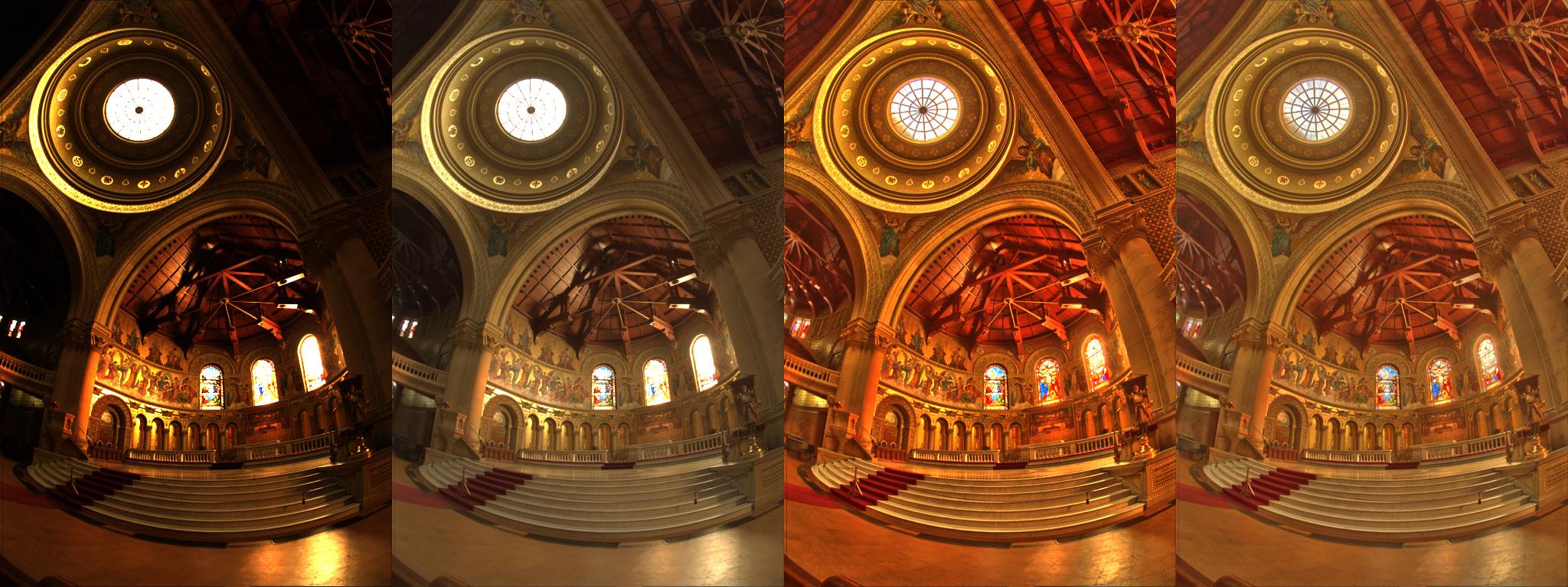
HDR images can also be used to create hyper-realistic and contrast enhanced LDR images. This paper describes a simple technique for increasing the contrast of images by using a local tonemapping operator, which effectively compresses the photo's dynamic range into a displayable format while still preserving detail and contrast. For 30 extra credit points, implement the method found in the paper and compare your results to other tonemapping operations (see example below for ideas). We provide you bilateral_filter function, but do not use any other third party code. You can find some example HDR images here, including the memorial church image used below.
From left to right: simple rescaling, rescaling+gamma correction, local tonemapping operator, local tonemapping+gamma correction.
Materials
Starter material for the project: Includes notebook, util codes, LDR mirror ball pictures, the resulting equirectangular HDR image, and a sample blender file for compositing.
Scoring and Deliverables
Use both words and images to show us what you've done please! See project instructions for submission details.
The core assignment is worth 100 points, as follows:
50 points for LDR-to-HDR merging
10 points for Data collection for 3 exposures (show the three images and a picture of the background/setting).
10 points for Naive merging. Show the estimated log irradiance image for all 3 exposures as well as the resulting merged log irradiance image. Explain how you computed this result.
10 points for Exposure Correction (accounting for under and over-exposed regions). Show the 3 estimated log irradiance images and the resulting merged log irradiance image. Give an explanation of how you computed this image.
15 points for Response Function estimation. Show the 3 estimated log irradiance images and the resulting merged log irradiance image. Additionally, plot the estimated function g; that is, plot pixel value vs g(pixel value) i.e. plt.plot(range(255), g).
5 points Under a heading "Irradiance Discussion", explain for each of the three methods (naive, exposure correction, response function estimation) whether (or in what conditions) the irradiance images for different exposures should be similar. To help you answer, examine a few pixels across the various exposures. Remember that g(Z) = ln(t) + ln(E), where Z are pixel values and t is the exposure time in seconds. For the first two stages, we haven't estimated g, so you can assume g(Z) = ln(Z).
10 points for the panoramic transformation and final equirectangular image and image-based light compositing result (including intermediate renderings).
5 points : Show the Normal image, Reflection image (R = X, G = Y, B = Z), and the Phi-Theta Image (spherical coordinate transformed image).
5 points : Show your final equirectangular HDR image, in a displayable range.
30 points Image-based object relighting result
15 points: Show the intermediate renderings (render with objects, render without objects, object mask).
15 points: Show your background image and final composited result.
10 points for quality of results and project page.
Include notebook that contains code for merging the LDR images into an HDR image, and your domain transformation code. It should be clear from the function names which is which (e.g., makehdr_naive, makehdr_exposed, makehdr_gsolve, perspective_transform"). You do not need to submit any blend files used to create your results.
You can also earn up to 90 extra points for the bells & whistles mentioned above (up to 20 for an additional image-based lighting result; 20 for additional domain transformations; 20 for photographer removal; 30 for implementing the local tonemapping operator of Durand and Dorsey). Describe bells and whistles under a separate heading and include relevant code/results.
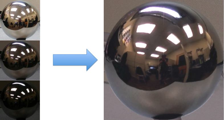 To the right are three pictures taken with different exposure times (1/24s, 1/60s, 1/120s) of a spherical mirror in my office. The rightmost image shows the HDR result (tonemapped for display). In this part of the project, you'll be creating your own HDR images. First, you need to collect the data.