Classifiers turn sets of input features into labels. At a very high level:
Classifiers can be used to classify static objects and to make decisions.
We've seen a naive Bayes classifier used to identify the type of text, e.g. label extracts such as the following as math text, news text, or historical document.
Let V be a particular set of vertices of cardinality n. How many different (simple, undirected) graphs are there with these n vertices? Here we will assume that we are naming the edges of the graph using a pair of vertices (so you cannot get new graphs by simply renaming edges). Briefly justify your answer. (from CS 173 study problems)
Senate Majority Leader Mitch McConnell did a round of interviews last week in which he said repealing Obamacare and making cuts to entitlement programs remain on his agenda. Democrats are already using his words against him. (from CNN, 21 October 2018)
Congress shall make no law respecting an establishment of religion, or prohibiting the free exercise thereof; or abridging the freedom of speech, or of the press; or the right of the people peaceably to assemble, and to petition the Government for a redress of grievances.
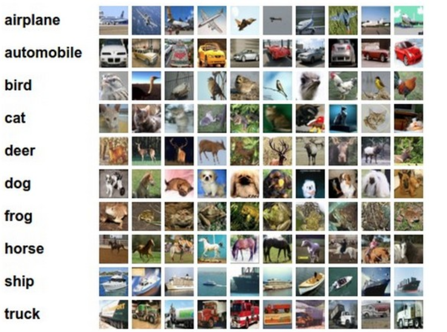
Classifiers can also be used label low-level input. For example, we can label what kind of object is in a picture. Or we can identify what phone has been said in each timeslice of a speech signal.
from Alex Krizhevsky's web page
"computer"
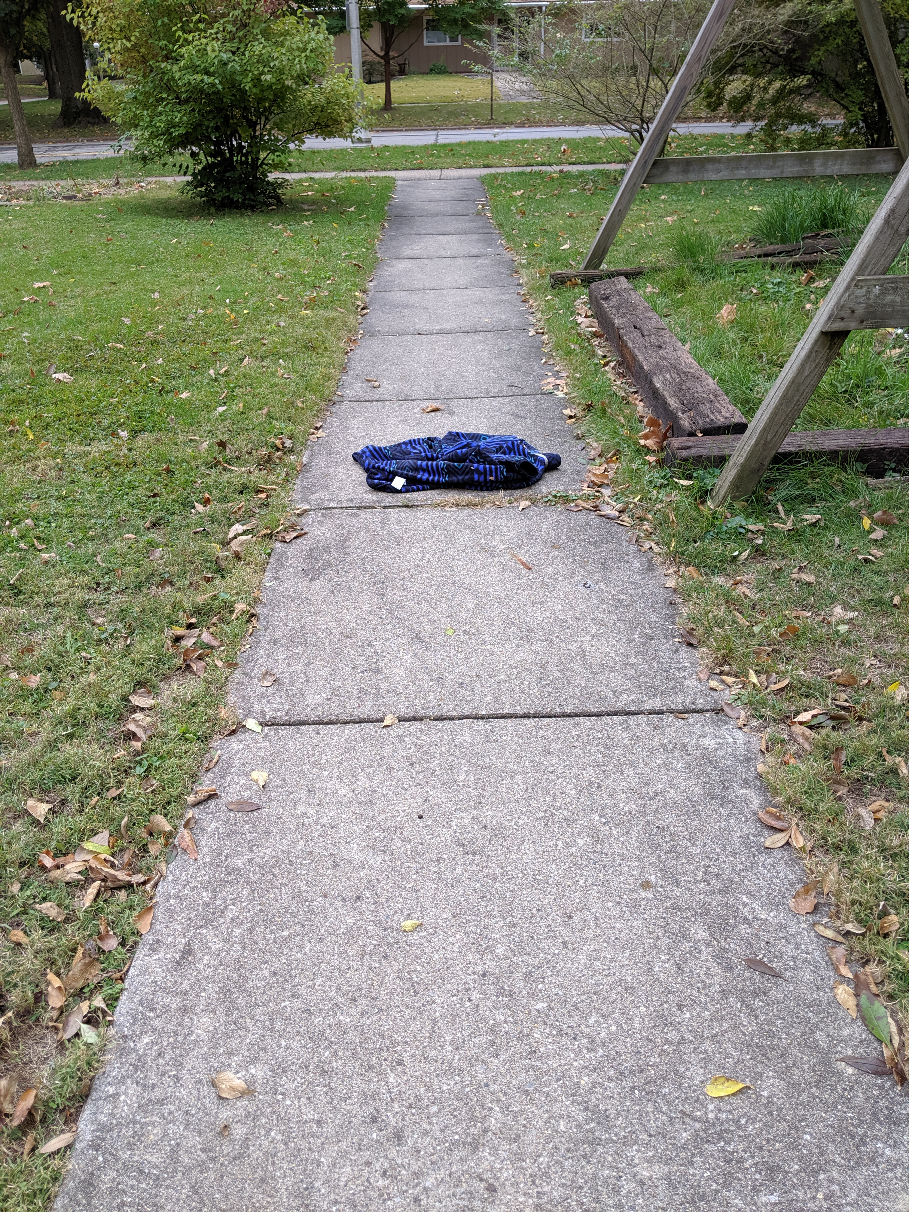
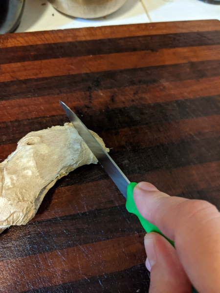
Classifiers can also be used to make decisions. For example, we might examine the state of a video game and decide whether to move left, move right, or jump. In the pictures below, we might want to decide if it's safe to move forwards along the path or predict what will happen to the piece of ginger.
Classifiers may also be used to make decisions internally to an AI system. Suppose that we have constructed the following parse tree and the next word we see is "Mary's".
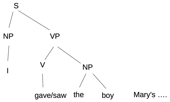
We have to decide how to attach "Mary's" into the parse tree. In "I gave the boy Mary's hat," "Mary's hat" will be attached to the VP as a direct object. In "I saw the boy Mary's going out with," the phrase "Mary's going out with" is a modifier on "boy." The right choice here depends on the verb (gave vs. saw) and lookahead at the words immediately following "Mary's".
Current algorithms require a clear (and fairly small) set of categories to classify into. That's largely what we'll assume in later lectures. But this assumption is problematic, and could create issues for deploying algorithms into the unconstrained real world.
For example, the four objects below are all quite similar, but nominally belong to three categories (peach, Asian pear, and two apples). How specific a label are we looking for, e.g. "fruit", "pear", or "Asian pear"? Should the two apples be given distinct labels, given that one is a Honeycrisp and one is a Granny Smith? Is the label "apple" correct for a plastic apple, or an apple core? Are some classification mistakes more/less acceptable than others? E.g. mislabelling the Asian pear as an apple seems better than calling it a banana, and a lot better than calling it a car.

What happens if we run into an unfamiliar type of object? Suppose, for example, that we have never seen an Asian pair. This problem comes up a lot, because people can be surprisingly dim about naming common objects, even in their first language. Do you know what a parsnip looks like? How about a plastron? Here is an amusing story about informant reliability from Robert M. Laughlin (1975, The Great Tzotzil Dictionary). In this situation, people often use the name of a familiar object, perhaps with a modifier, e.g. a parsnip might be "like a white carrot but it tastes different." Or they may identify the general type of object, e.g. "vegetable."
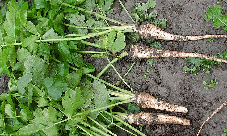
parsnips from Wikipedia
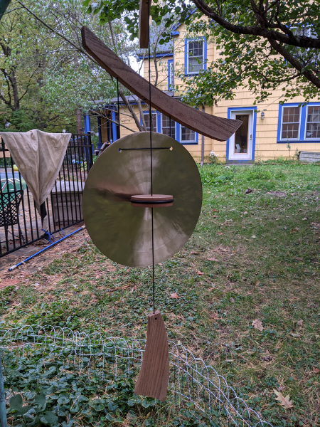
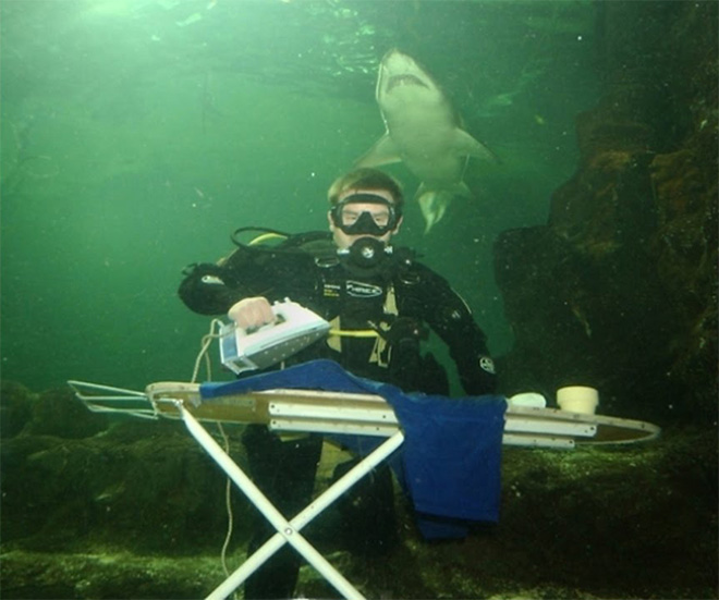
Some unfamiliar objects and activities can be described in terms of their components. E.g. the wind chime below has a big metal disk and some mysterious wood parts. The middle picture below is "a house with a shark sticking out of it." The bottom picture depicts ironing under water.
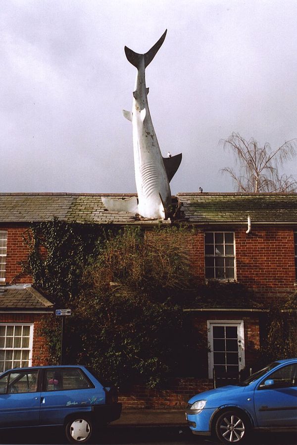
shark from
Wikipedia,
diver from
Sad and Useless
When labelling objects, people use context as well as intrinsic properties. This can be particularly important when naming a type of object whose appearance can vary substantially, e.g. the vases in the picture below.

A famous experiment by William Labov (1975, "The boundaries of words and their meanings") showed that the relative probabilities of two labels (e.g. cup vs. bowl) change gradually as properties (e.g. aspect ratio) are varied. For example, the tall container with no handle (left) is probably a vase. The round container on a stem (right) is probably a glass. But what are the two in the middle?

The very narrow container was sold as a vase. But filling it with liquid would encourage people to call it a glass (perhaps for a fancy liquor). Installing flowers in the narrow wine glass makes it seem more like a vase. And you probably didn't worry when I called it a "vase" above. The graph below (from the original paper) shows that imagining a food context makes the same picture more likely to be labelled as a bowl rather than a cup.

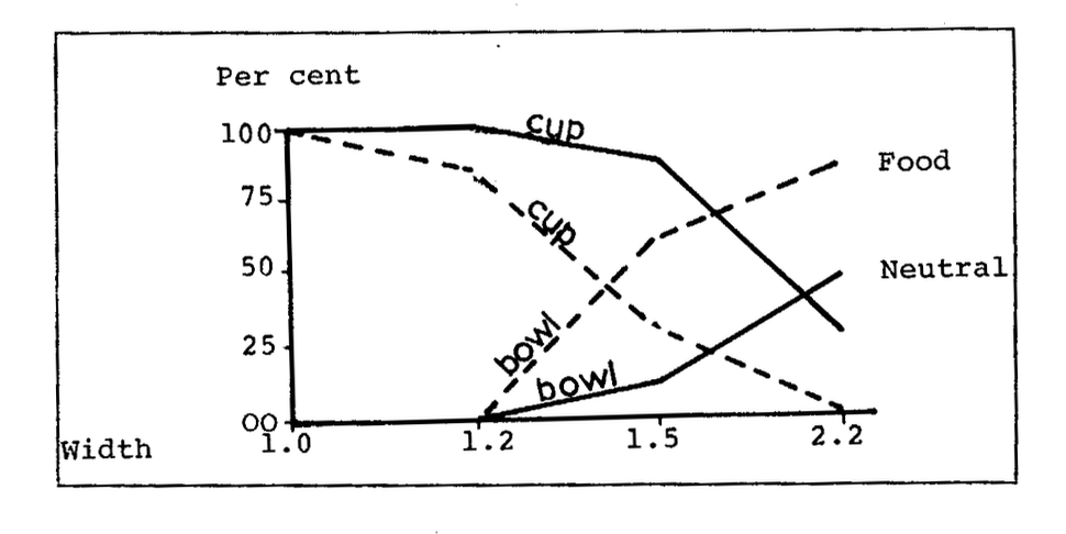
from William Labov (1975)
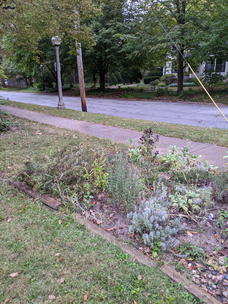
With complex scenes, it's not clear how many objects to explicitly call out. E.g. is the picture below showing a garden or a street? Are we supposed to be labelling each plant? Should we mark out the street lamp? The sidewalk?
When you're talking to another human, it's much more clear what aspects of the scene are important. First, there is usually some larger context that the conversation fits into (e.g. "gardening" or "traffic"). Second, people look at things they are interested in, e.g. compare the two pictures below. People have very strong ability to track another person's gaze as we watch what they are doing. Because of their close association with humans, the same applies to dogs. Using gaze to identify interest is believed to be an integral part of how children associate names with objects. Lack of appropriate eye contact is one reason that conversations feel glitchy on video conferencing systems.


It's tempting to see this problem as specific to computer vision. However, there are similar examples from other domains. E.g. in natural language processing, it's common to encounter new words. These can be unfamiliar proper nouns (e.g. "Gauteng", "covid"). Or they may be similar to familiar words, e.g. typos ("coputer") or new compounds ("astroboffin") or melds ("brexit", "splinch"). Phone recognition may involve more or less detail and mistakes may be minor (e.g. "t" vs. "d") or major (e.g. "t" vs. "a").
People use prosodic features (e.g. length, stress) to indicate which words are most important for the listener to pay attention to. And we use context to decide which meaning of a word is appropriate e.g. "banks" is interpreted very differently in "The pilot banks his airplane." vs. "Harvey banks at First Financial."
Classifier systems often have several stages. "Deep" models typically have more distinct layers. Each layer in a deep model does a simpler task and the representation type more changes gradually from layer to layer.
| speech recognizer | object identification | scene reconstruction | parsing | word meaning | |
|---|---|---|---|---|---|
| raw input | waveform | image | images | text | text |
| low-level features | MFCC features | edges, colors | corners, SIFT features | stem, suffixes word bigrams |
word neighbors |
| low-level labels | phone probabilities | local object ID | raw matchpoints | POS tags | word embeddings |
| output labels | word sequence | image description | scene geometry | parse tree | word classes |
Representations for the raw input objects (or sometimes the low-level features) have a large number of bits. E.g. a color image with 1000x1000 pixels, each containing three color values. Early processing often tries to reduce the dimensionality by picking out a smaller set of "most important" dimensions. This may be accomplished by linear algebra (e.g. principal components analysis) or by classifiers (e.g. word embedding algorithms).
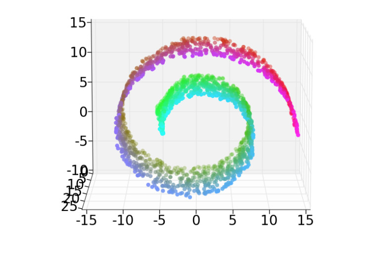
When the data is known to live on a subset of lower dimension, vectors may be mapped onto this subset by so-called "manifold learning" algorithms. For example, color is used to enclose class (output label). Distance along the spiral correctly encodes class similarity. Straight-line distance in 3D does the wrong thing: some red-green pairs of points are closer than some red-red pairs.
There are two basic approaches to each stage of processing:
Many real systems are a mix of the two. A likely architecture for a speech recognizer (e.g. the Kaldi system) would start by converting the raw signal to MFCC features, then use a neural net to identify phones, then use an HMM-type decoder to extract the most likely word sequence.
There are three basic types of classifiers with learned parameters. We've already seen the first type and we're about to move onto the other three
Classifiers typically have a number of overt variables that can be manipulated to produce the best outputs. These fall into two types:
Researchers also tune the structure of the model.
It is now common to use automated scripts to tune hyperparameters and some aspects of the model structure. Tuning these additional values is a big reason why state-of-the-art neural nets are so expensive to tune. All of these tunable values should be considered when assessing whether the model could potentially be over-fit to the training/development data, and therefore might not generalize well to slightly different test data.
Training and testing can be interleaved to varying extents:
Incremental training is typically used by algorithms that must interact with the world before they have finished learning. E.g. children need to interact with their parents from birth, long before their language skills are fully mature. Sometimes interaction is to get their training data. E.g. a video game player may need to play experimental games. Incremental training algorithms are typically evaluated based on their performance towards the end of training.
Traditionally, most classifiers used "supervised" training. That is, someone gives the learning algorithm a set of training examples, together with correct ("gold") output for each one. This is very convenient, and it is the setting in which we'll learn classifier techniques. But this only works when you have enough labelled training data. Usually the amount of training data is inadequate, because manual annotations are very slow to produce.
Moreover, labelled data is always noisy. Algorithms must be robust to annotation mistakes. It may be impossible to reach 100% accuracy because the gold standard answers aren't entirely correct.
Finally, large quantities of correct answers may be available only for the system as a whole, not for individual layers. Marking up correct answers for intermediate layers frequently requires expert knowledge, so cannot easily be farmed out to students or internet workers.
Researchers have a used a number of methods to work around lack of explicit labelled training data. For example, current neural net software lets us train the entire multi-layer as a unit. Then we need correct outputs only for the final layer. This type of training optimizes the early layers only for this specific task. However, it may be possible to quickly adapt this "pre-trained" layer for use in another task, using only a modest amount of new training data for the new task.
For example, the image colorization algorithm shown below learns how to add color to black and white images. The features it exploits in the monochrome images can also (as it turns out) be used for object tracking.
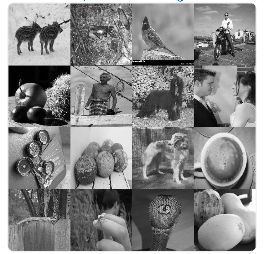
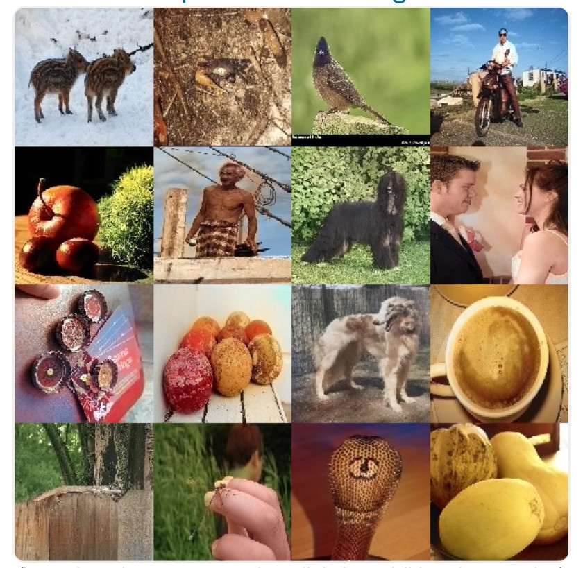
from Zhang, Isola, Efros
Colorful Image Colorization
For this colorization task, the training pairs were produced by removing color from
color pictures. That is, we subtracted information and learned to restore it.
This trick for producing training pairs has been used elsewhere. For example, the
BERT system trains natural language models by masking off words in training sentences,
and learning to predict what they were. Similarly, the pictures below illustrate
that we can learn to fill in missing image content, by creating training images with
part of the content masked off.
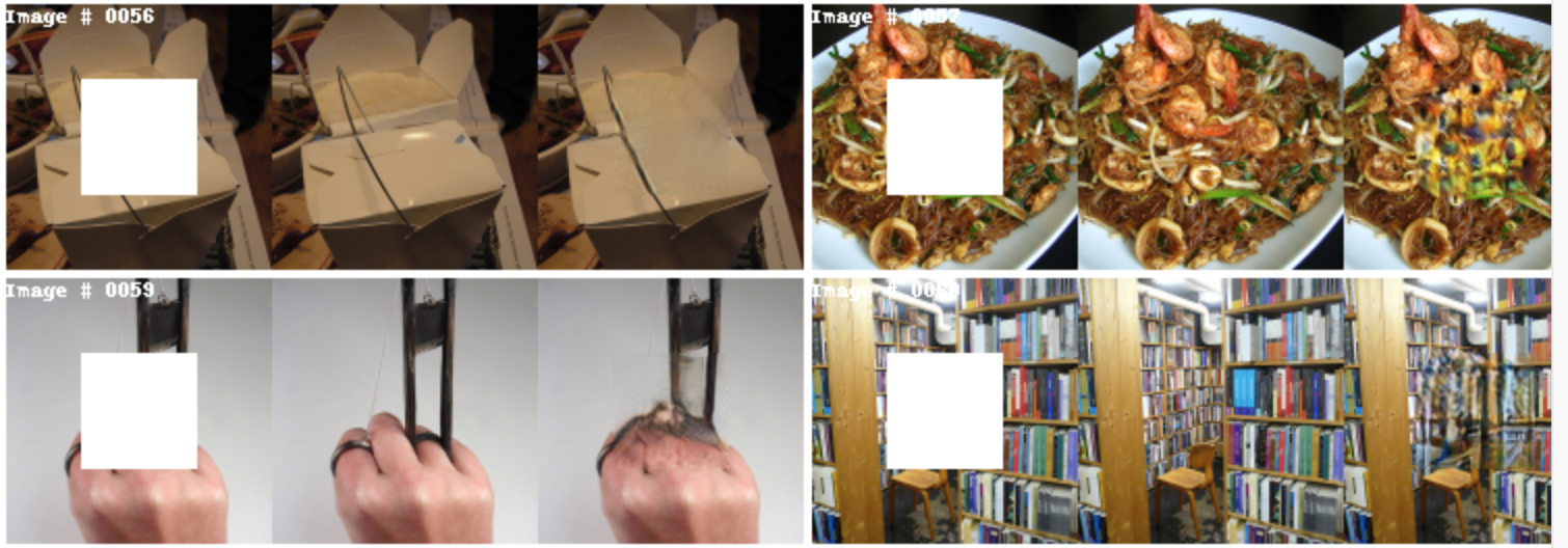
from Pathak et al. "Context Encoders: Feature Learning by
Inpainting"
Another approach is self-supervision, in which the learner experiments with the world to find out new information. Examples of self-supervision include
The main challenge for self-supervised methods is designing ways for a robot to interact with a real, or at least realistic, world without making it too easy for the robot to break things, injury itself, or hurt people.
"Semi-supervised" algorithms extract patterns from unannotated data, combining this with limited amounts of annotated data. For example, a translation algorithm needs some parallel data from the two languages to create rough translations. The output can be made more fluent by using unannotated data to learn more about what word patterns are/aren't appropriate for the output language. Similarly, we can take observed pauses in speech and extrapolate the full set of locations where it is appropriate to pause (i.e. word boundaries).
"Unsupervised" algorithms extract patterns entirely from unannotated data. These are much less common than semi-supervised methods. Sometimes so-called unsupervised methos actually have some implicit supervision (e.g. sentence boundaries for a parsing algorithm). Sometimes they are based on very strong theoretical assumptions about how the input must be structured.
Here's a schematic representation of English vowels (from Wikipedia). From this, you might reasonable expect to experimental data to look like several tight clusters of points, well-separated. If that were true, then classification would be easy: model each cluster with a regeion of simple shape (e.g. ellipse), compare a new sample to these region, and pick the one that contains it.
However, experimental datapoints for these vowels (even after some normalization) actually look more like the following. If we can't improve the picture by clever normalization (sometimes possible), we need to use more robust methods of classification.

(These are the tirst two formants of English vowels by 50 British speakers, normalized by the mean and standard deviation of each speaker's productions. From the Experimental Phonetics course PALSG304 at UCL.)
Another way to classify an input example is to find the most similar training example and copy its label.
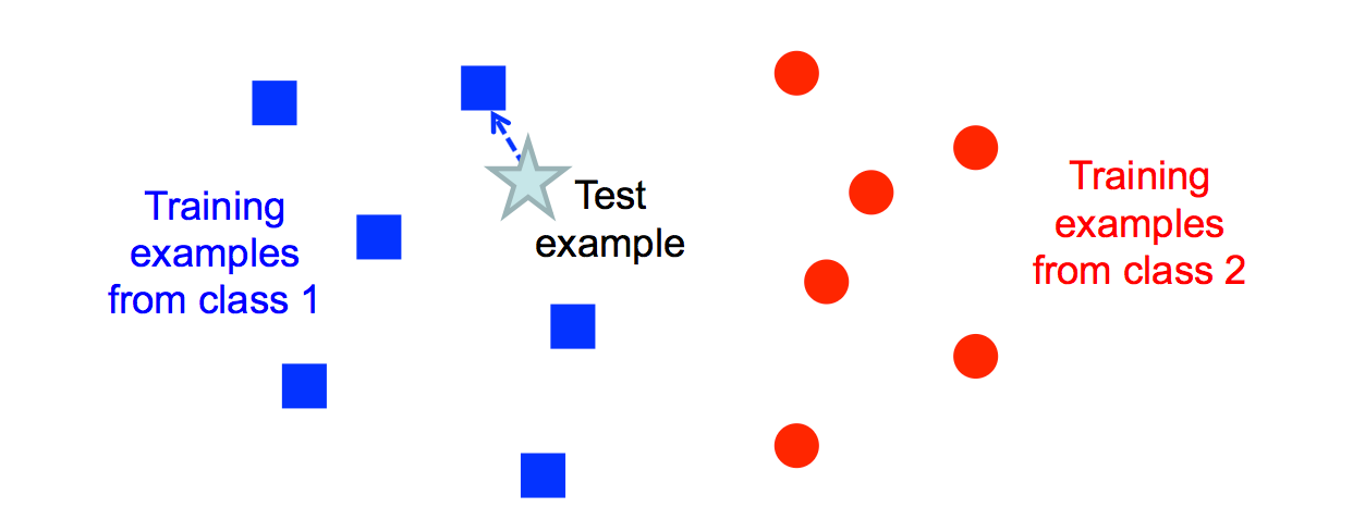
from Lana Lazebnik
This "nearest neighbor" method is prone to overfitting, especially if the data is messy and so examples from different classes are somewhat intermixed. However, performance can be greatly improved by finding the k nearest neighbors for some small value of k (e.g. 5-10).
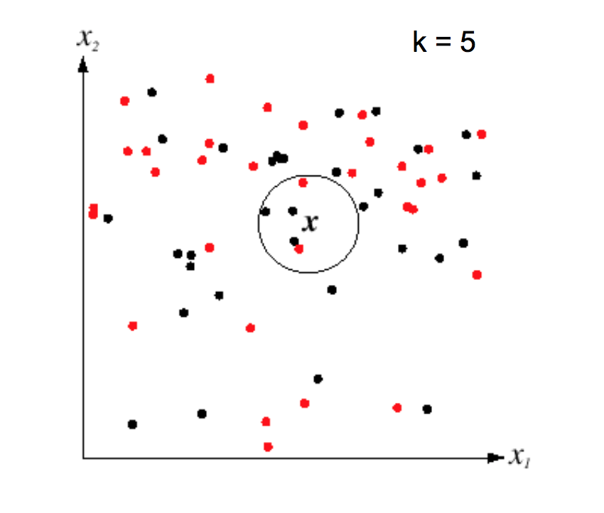
from Lana Lazebnik
K nearest neighbors can model complex patterns of data, as in the following picture. Notice that larger values of k smooth the classifier regions, making it less likely that we're overfitting to the training data.
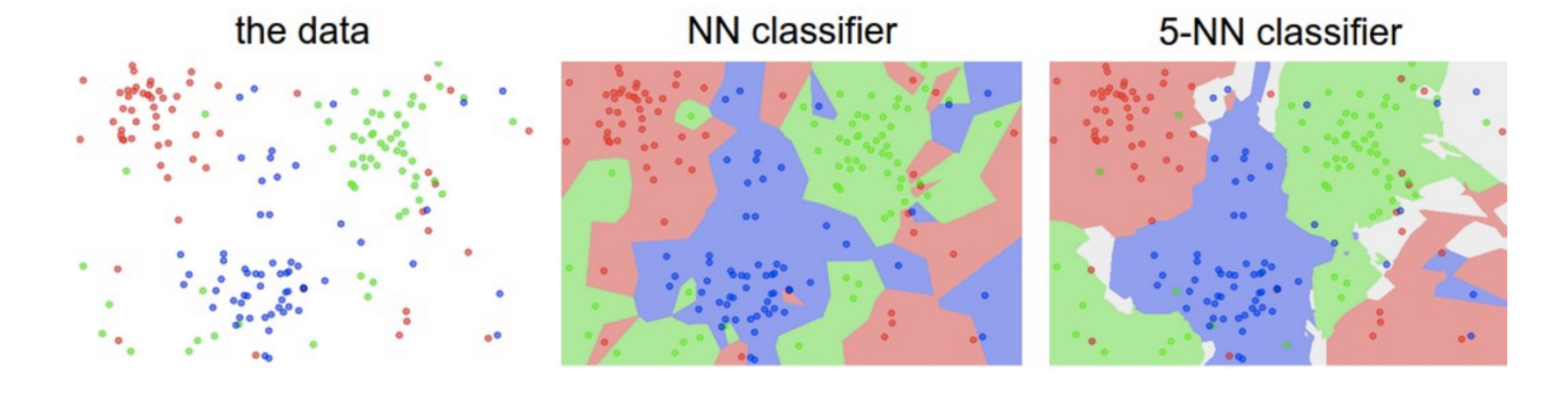
from Andrej Karpathy
A limitation of k nearest neighbors is that the algorithm requires us to remember all the training examples, so it takes a lot of memory if we have a lot of training data. Moreover, the obvious algorithm for classifying an input image X requires computing the distance from X to every stored image. In low dimensions, a k-D tree can be used to find efficiently find the nearest neighbors for an input example. However, efficiently handling higher dimensions is more tricky and beyond the scope of this course.
This method can be applied to somewhat more complex types of examples. Consider the CFAR-10 dataset below. (Pictures are from Andrej Karpathy cs231n course notes.) Each image is 32 by 32, with 3 color values at each pixel. So we have 3072 feature values for each example image.
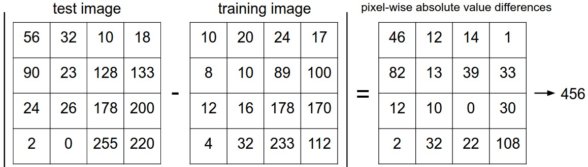
We can calculate the distance between two examples by subtracting corresponding feature values. Here is a picture of how this works for a 4x4 toy image.
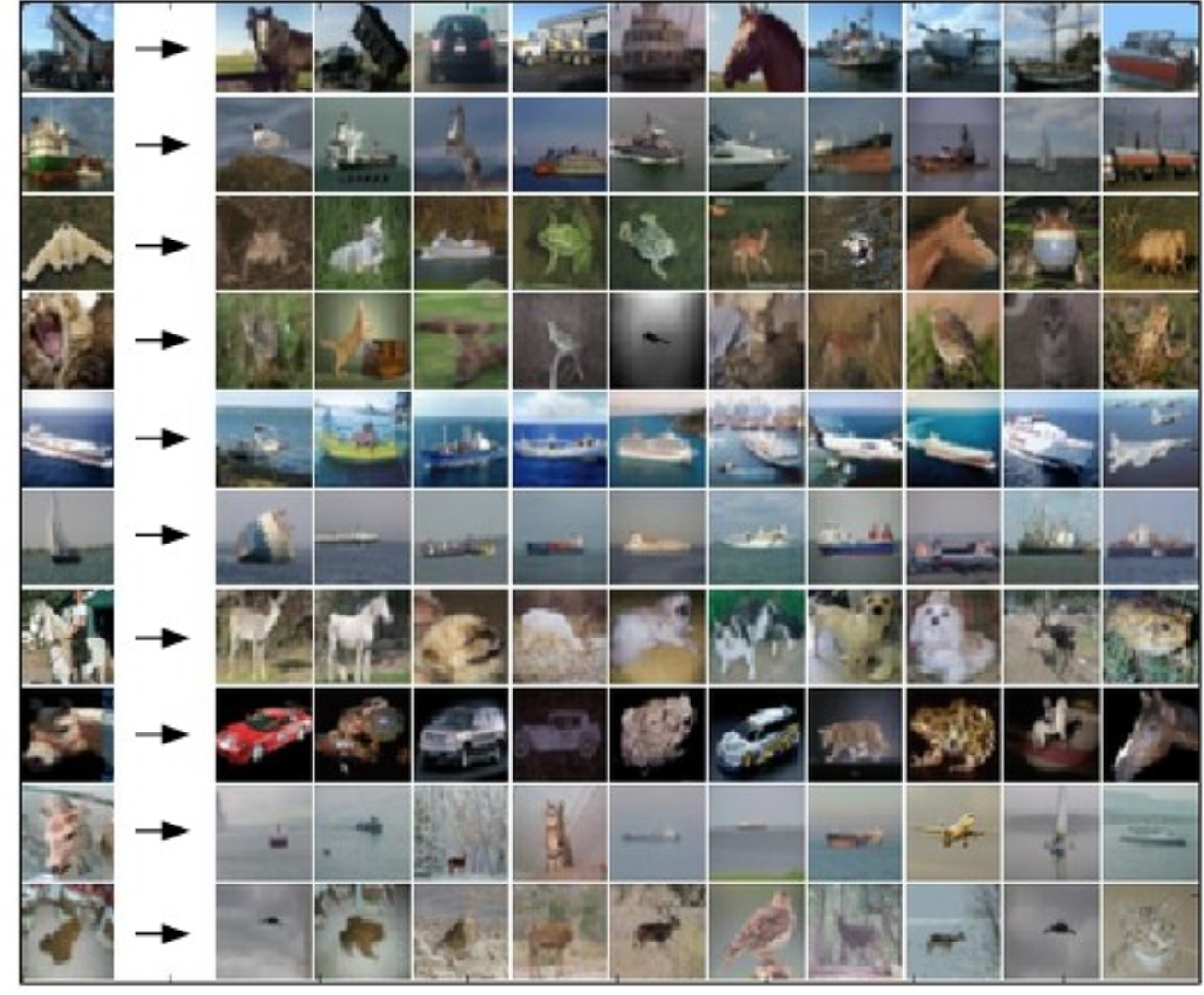
The following picture shows how some sample test images map to their 10 nearest neighbors.
More precisely, suppose that \(\vec{x}\) and \(\vec{y}\) are two feature vectors (e.g. pixel values for two images). Then there are two different simple ways to calculate the distance between two feature vectors:
As we saw with A* search for robot motion planning, the best choice depends on the details of your dataset. The L1 norm is less sensitive to outlier values. The L2 norm is continuous and differentiable, which can be handy for certain mathematical derivations.
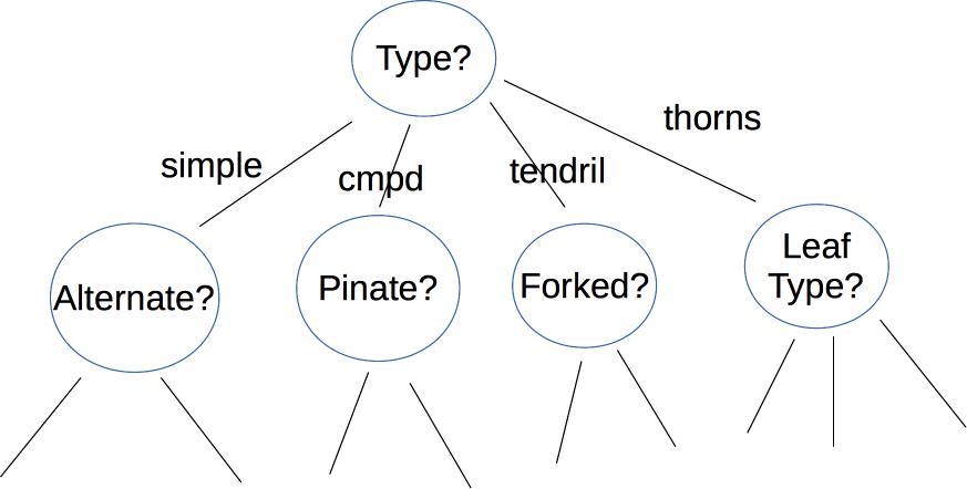
A decision tree makes its decision by asking a series of questions. For example, here is a a decision tree user interface for identifying vines (by Mara Cohen, Brandeis University). The features, in this case, are macroscopic properties of the vine that are easy for a human to determine, e.g. whether it has thorns. The top levels of this tree look like
Similar decision trees can appear inside AI systems. For example, here's a decision tree from a system by Ferrer, Shriberg, and Stolcke (2003) that detects when a user has finished speaking using prosodic features. This system runs its decision tree on each section of the speech (a frame) until it decides that the speaker has ended. Such a system would be used to decide when an AI system should attempt to take its own turn speaking, e.g. answer the human's questions.
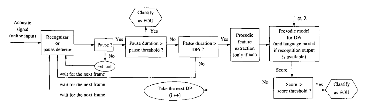
Depending on the application, the nodes of the tree may ask yes/no questions, multiple choice (e.g. simple vs. complex vs. tendril vs thorns), or set a threshold on a continuous space of values (e.g. is the tree below or above 6' tall?). The output label may be binary (e.g. is this poisonous?), from a small set (edible, other non-poisonous, poisonous), or from a large set (e.g. all vines found in Massachusetts). The strength of decision trees lies in this ability to use a variety of different sorts of features, not limited to well-behaved numbers.
Here's an example of a tree created by thresholding two continuous variable values (from David Forsyth, Applied Machine Learning). Notice that the split on the second variable (x) is different for the two main branches.
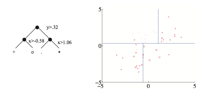
Each node in the tree represents a pool of examples. Ideally, each leaf node contains only objects of the same type. However, that isn't always true if the classes aren't cleanly distinguished by the available features (see the vowel picture above). So, when we reach a leaf node, the algorithm returns the most frequent label in its pool.
If we have enough decision levels in our tree, we can force each pool to contain objects of only one type. However, this is not a wise decision. Deep trees are difficult to construct (see the algorithm in Russell and Norvig) and prone to overfitting their training data. It is more effective to create a "random forest", i.e. a set of shallow trees (bounded depth) and have these trees vote on the best label to return. The set of shallow trees is created by choosing variables and possible split locations randomly.
Whether we're building a deep or shallow tree, some possible splits are a bad idea. For example, the righthand split leaves us with two half-size pools that are no more useful than the original big pool.
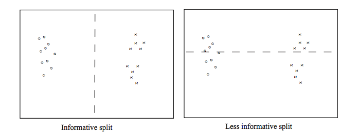
From David Forsyth, Applied Machine Learning.
A good split should produce subpools that are less diverse than the original pool. If we're choosing between two candidate splits (e.g. two thresholds for the same numerical variable), it's better to pick the one that produces subpools that are more uniform. Diversity/uniformity is measured using entropy.
Suppose that we are trying to compress English text, by translating each character into a string of bits. We'll get better compression if more frequent characters are given shorter bit strings. For example, the table below shows the frequencies and Huffman codes for letters in a toy example from Wikipedia.
| Char | Freq | Code | Char | Freq | Code | Char | Freq | Code | Char | Freq | Code | Char | Freq | Code | Char | Freq | Code | Char | Freq | Code |
|---|---|---|---|---|---|---|---|---|---|---|---|---|---|---|---|---|---|---|---|---|
| space | 7 | 111 | a | 4 | 010 | e | 4 | 000 | ||||||||||||
| f | 3 | 1101 | h | 2 | 1010 | i | 2 | 1000 | m | 2 | 0111 | n | 2 | 0010 | s | 2 | 1011 | t | 2 | 0110 |
| l | 1 | 11001 | o | 1 | 00110 | p | 1 | 10011 | r | 1 | 11000 | u | 1 | 00111 | x | 1 | 10010 |
Suppose that we have a (finite) set of letter types S. Suppose that M is a finite list of letters from S, with each letter type (e.g. "e") possibly included more than once in M. Each letter type c has a probability P(c) (i.e. its fraction of the members of M). An optimal compression scheme would require \(\log(\frac{1}{P(c)}) \) bits in each code. (All logs in this discussion are base 2.)
To understand why this is plausible, suppose that all the characters have the same probability. That means that our collection contains \(\frac{1}{P(c)} \) different characters. So we need \(\frac{1}{P(c)} \) different codes, therefore \(\log(\frac{1}{P(c)}) \) bits in each code. For example, suppose S has 8 types of letter and M contains five of each. Then we'll need 8 distinct codes (one per letter), so each code must have 3 bits. This squares with the fact that each letter has probability 1/8 and \(\log(\frac{1}{P(c)}) = \log(\frac{1}{1/8}) = \log(8) = 3 \).
The entropy of the list M is the average number of bits per character when we replace the letters in M with their codes. To compute this, we average the lengths of the codes, weighting the contribution of each letter c by its probability P(c). This give us
\( H(M) = \sum_{c \in S} P(c) \log(\frac{1}{P(c)}) \)
Recall that \(\log(\frac{1}{P(c)}) = -\log(P(c))\). Applying this, we get the standard form of the entropy definition.
\( H(M) = - \sum_{c \in S} P(c) \log(P(c)) \)
In practice, good compression schemes don't operate on individual characters and also they don't achieve this theoretical optimum bit rate. However, entropy is a very good way to measure the homogeneity of a collection of discrete values, such as the values in the decision tree pools.
For more information, look up Shannon's source coding theorem.
