
From Wikipedia
Nov 13, 12:15pm CST, a bug that affects early_check and
the checkpoints that check.py uses has been fixed. Please
re-download the template and double-check
your code against the updated autograder.
From
Wikipedia
Snake is a famous video game originated in the 1976 arcade game Blockade. The player uses up, down, left and right to control the snake which grows in length (when it eats the food pellet), with the snake body and walls around the environment being the primary obstacle. In this assignment, you will train an AI agent using reinforcement learning to play a simple version of the game snake. You will implement a TD version of the Q-learning algorithm.
The external libraries required for this project are
numpy and pygame. To play the game yourself
and get acquainted with it, you can run
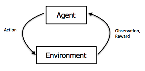
python mp11_12.py --human For us to program an AI that plays Snake by itself, we first need to understand how the game can be viewed from the lens of reinforcement learning (RL). Broadly, RL can be completely described as an agent acting in an environment.
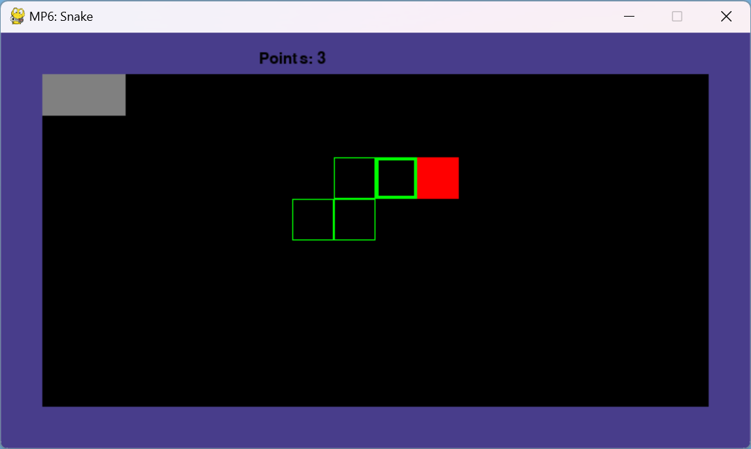
Our environment is the game board, visualized in the picture above. The green rectangle is the snake agent, and the red rectangle is the food pellet. The snake head is marked with a thicker border for easier recognition. In utils.py, We define some constants that control the pixel-wise sizes of everything:
1.1 x 1.1 per frame.2 x 1, not necessarily in the
top left corner.In the above picture, we have set our game board to be 18x10, with size 1 walls, size 1 snake body, a rock at (1,1), and food. Therefore, we can treat the valid operating space of the snake to be a grid of blocks surrounded by a wall on each side. Note that the our coordinate system has the top left is (1,1). In other words, (2,2) is below and to the right of (1,1).
Implementation Tips: when computing quantities such
as collisions with walls, use the top left corner of each “grid
block” for its overall position. Also, check utils.py
before hard coding any constants; if it is provided there, use the
constant and not a hard coded value.
The objective of the game is to move the snake around the grid to collect food pellets. Every time the snake/agent eats a food pellet, the points increase by 1 and the snake’s body grows one segment. When a food pellet is eaten, a new food pellet is generated randomly on the board.
The game ends when the snake dies, after which the environment rests.
The snake dies if the snake head touches any of the 4 walls, or if it
touches its own body (which occurs if the head goes backwards). The
snake will also die after taking \(8
*\) DISPLAY_SIZE steps without food. The
DISPLAY_SIZE equals to the width times the height of the
display area (18 x 10 = 180 in the above example).
With our environment defined, we can now move on to the agent. The agent operates in the environment by defining a Markov Decision Process (MDP), which contains
Each state in the MDP is a tuple
(food_dir_x, food_dir_y, adjoining_wall_x, adjoining_wall_y, adjoining_body_top, adjoining_body_bottom, adjoining_body_left, adjoining_body_right).
[food_dir_x, food_dir_y] indicates
the direction of food relative to the snake head. Each takes 3 possible
values:
food_dir_x: 0
(same coords on x axis), 1 (food on snake head left),
2 (food on snake head right)
food_dir_y: 0
(same coords on y axis), 1 (food on snake head top),
2 (food on snake head bottom)
[adjoining_wall_x, adjoining_wall_y]
indicates whether there is a wall or a rock next to the snake head. Each
takes 3 possible values:
adjoining_wall_x:
0 (no adjoining wall/rock on x axis),
1 (wall/rock on snake head left, or wall/rock
on both snake head left and right), 2 (wall/rock on
snake head right)
adjoining_wall_y:
0 (no adjoining wall/rock on y axis),
1 (wall/rock on snake head top or wall/rock on
both snake head top and bottom), 2 (wall/rock on snake
head bottom)
To clarify: for both
adjoining_wall_xandadjoining_wall_y, the priority goes(adjoining_wall_[x/y] = 1) > (adjoining_wall_[x/y]=2). For example, when there is a rock or a wall both above and below the head, setadjoining_wall_y=1.
Note that
[adjoining_wall_x, adjoining_wall_y] = [0, 0]
can also occur when the snake runs out of the board boundaries.
[adjoining_body_top, adjoining_body_bottom, adjoining_body_left, adjoining_body_right]
checks if a grid next to the snake head contains the snake body. Each
takes 2 possible values:
adjoining_body_top: 1
(adjoining top square has snake body), 0
(otherwise)adjoining_body_bottom:
1 (adjoining bottom square has snake body),
0 (otherwise)adjoining_body_left:
1 (adjoining left square has snake body),
0 (otherwise)adjoining_body_right:
1 (adjoining right square has snake body),
0 (otherwise)In each timestep, your agent will choose an action from the set
{UP, DOWN, LEFT, RIGHT}. You should use the respective
variables defined in utils.py for these quantities.
In each timestep, your agent will receive a reward from the environment after taking an action. The rewards are:
You will create a snake agent that learns how to get as many food pellets as possible without dying, which corresponds to maximizing the reward of the agent. In order to do this, we will use the Q-learning algorithm. Your task is to implement the TD Q-learning algorithm and train it on the MDP outlined above.
In Q-learning, instead of explicitly learning a representation for transition probabilities between states, we let the agent observe its environment, choose an action, and obtain some reward. In theory, after enough iterations, the agent will implicitly learn the value for being in a state and taking an action. We refer to this quantity as the Q-value for the state-action pair.
Explictly, our agent interacts with it’s environment in the following feedback loop:
Often, the notations for the current state \(s_t\) and next state \(s_{t+1}\) are written as \(s\) and \(s'\), respectively. Same for the current action \(a\) and next action \(a'\).
The Q update formula is:

where \(\gamma\) is the Temporal-Difference (TD) hyperparameter discounting future rewards, and
\[ \alpha = \frac{C}{C + N(s,a)} \]
is the learning rate controlling how much our Q estimate should change with each update. Unpacking this equation: \(C\) is a hyperparameter, and \(N(s,a)\) is the number of times the agent has been in state \(s\) and taken action \(a\). As you can see, the learning rate decays as we visit a state-action pair more often.
With its current estimate of the Q-states, the agent must choose an “optimal” action to take. However, reinforcement learning is a balancing act between exploration (visiting new states to learn their Q-values) and greed (choosing the action with the highest Q-value). Thus, during training, we use an exploration policy defined below:
\[ a^* = \text{argmax}_{a}\ \ f(Q(s,a), N(s,a))\] \[ f(Q(s,a), N(s,a)) = \begin{cases}1 & N(s,a) < Ne \\ Q(s,a) & else\end{cases}\]
where \(Ne\) is a hyperparameter. Intuitively, if an action hasn’t been explored enough times (when \(N(s,a) < Ne\)), the exploration policy chooses that action regardless of its Q-value. If there are no such actions, the policy chooses the action with the highest Q value. This policy forces the agent to visit each state and action at least \(Ne\) times.
Implementation Note: If there is a tie among
actions, break it according to the priority order
RIGHT > LEFT > DOWN > UP.
When implementing Q-learning as described above, you will need to
read and update Q and N-values. For this, we have created appropriately
large tables that are defined in the Agent constructor in agent.py. You
should read and write from these tables, as we will be grading part of
your implementation on their contents. The order of parameters in the Q
and N-tables are mentioned at the end of these instructions.
Alternatively, you can look in the body of create_q_table()
in utils.py to see how they are initialized.
Update the N-table before the Q-table, so that the learning rate for the very first update will be a little less than 1. This is an arbitrary choice (as long as the learning rate decays with time we effectively get the same result), but it is necessary to get full-credit on the autograder. To make your code cleaner, we recommend doing the N and Q-updates right next to each other in the code.
When testing, your agent no longer needs to update either table. Your agent just needs to observe its environment, generate the appropriate state, and choose the optimal action without the exploration function.
Implementation Note: Don’t forget the edge case for
updating your Q and N tables when \(t=0\). At \(t =
0\), both \(s\) and \(a\) will be None. In that
case, is there anything for us to update the Q and N-tables with? Only
at \(t = 1\) will \(s\) and \(a\) correspond to a state and action for
which you need to update the tables.
Implementation Note: When the agent “dies”, any arbitrary action can be chosen as the game will be reset before the action can be taken. This does not need to be recorded in the Q and N tables. But, you will still need to update Q and N for the action you just took that caused the death.
Before you start implementing the Q-learning algorithm, we recommend that you run the following tests to make sure the state are generated (discretized) correctly and your Q and N-tables are being updated correctly. This will be the primary task of MP11.
You can test this without implementing the act function.
In this test, we give several specific environments to check your state
generation and specific action sets to check if your Q and N-tables
match ours.
Test data are stored in test_data.py. We have provided the expected Q and N-tables of these tests in the template code’s data/early_check folder. The file game_1_N.npy and game_1.npy correspond to the first game, game_2_N.npy and game_2.npy to the second game, and so on.
All other parameters are the same as the default values in utils.py. To trigger the test, run:
python mp11_12.py --early_checkThe autograder will perform early checking for MP11, and train and test your agent given a certain set of parameters for MP12.
Some of these commands will be more relevant to MP12, but we include them for your reference here.
To see the available parameters you can set for the game, run:
python mp11_12.py --helpTo train and test your agent, run:
python mp11_12.py [parameters]To see more examples, you can take a look at MP12.
This will train the agent, test it, and save a local copy of your Q and N-tables in checkpoint.npy and checkpoint_N.npy, respectively.
By default, it will train your agent for 10,000 games and test it for
1000, though you can change these by modifying the
--train-episodes and --test-episodes arguments
appropriately. In addition, it will also display some example games of
your trained agent at the end! (If you don’t want this to happen, just
change the --show-episodes argument to 0)
You will not be tested on parameter tuning to achieve a high number of points. The autograder will pass in our choice of hyperparameter values. (So do not hard code them!) If you have implemented Q-learning correctly, you should pass all the tests with full credit. However, for fun, we recommend playing around with the hyperparameters to see how well you can train your agent!
Trained Agent
The file template.zip contains the supplied code (described below) and the debugging examples described above.
Do not import any non-standard libraries except pygame and numpy
Use numpy version <= 1.21.3.
mp11_12.py - This is the main file that starts the program. This file runs the snake game with your implemented agent acting in it. The code runs a number of training games, then a number of testing games, and then displays example games at the end.
snake.py - This file defines the snake environment and creates the GUI for the game.
utils.py - This file defines environment constants as defined above and contains the functions to save and load models.
agent.py This is the file where you will be doing all of your work. This file contains the Agent class. This is the agent you will implement to act in the snake environment.
You should submit the file agent.py on Gradescope.
For MP11, you are only required to implement
generate_state(self, environment),
update_q(self, s, a, r, s_prime) and
update_n(self, state, action). The function
act(self, environment, points, dead) is left for MP12.
Inside agent.py, you will find the following
variables/methods of the Agent class useful:
self._train, self._test: These
boolean flags denote whether the agent is in train or test mode. In
train mode, the agent should explore (based on the exploration function)
and exploit based on the Q table. In test mode, the agent should purely
exploit and always take the best action. You may assume that these
variables are set appropriately. You do not need to change
them.
self.Q, self.N: These numpy
matrices hold the Q and N-tables, respectively. They are both of shape
(NUM_FOOD_DIR_X, NUM_FOOD_DIR_Y, NUM_ADJOINING_WALL_X_STATES, NUM_ADJOINING_WALL_Y_STATES, NUM_ADJOINING_BODY_TOP_STATES, NUM_ADJOINING_BODY_BOTTOM_STATES, NUM_ADJOINING_BODY_LEFT_STATES, NUM_ADJOINING_BODY_RIGHT_STATES,NUM_ACTIONS)
self.Ne, self.C, self.gamma:
Self-explanatory hyperparameters
self.reset(): This function resets
the environment from the agent’s perspective and should be run when the
agent dies.
self.points, self.s, self.a: These
variables should be used to store the points, state, and action,
respectively, for bookkeeping. That is, they will be helpful in
computing whether a new food pellet has been eaten, in addition to
storing previous state-action pairs that will be useful when
doing Q-value updates.
act(environment, points, dead):
This is the main function you will implement in MP12
and is called repeatedly by mp11_12.py while games are
being run. You do not need to implement this for MP11. The
--early_check flag will account for this.
update_n(self, state, action):
Update the N-table. See self.N and the section Q-learning agent.
update_q(self, s, a, r, s_prime):
Update the Q-table. See self.Q and the section Q-learning agent.
generate_state(self, environment):
Discretizes the state, using the environment, which is later used in the
Q-learning computation.