 Lecture 12: Probability
 Mulberry trees have edible berries and are critical for raising silkworms, The picture above shows a silk mill from a brief attempt (around 1834) to establish a silk industry in Northampton Massachusetts. But would you be able to tell a mulberry leaf from a birch leaf (below)? How would you even go about describing how they look different?
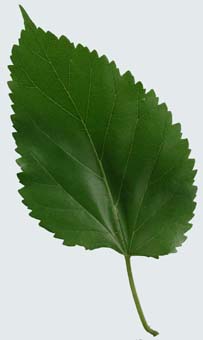
Which is mulberry and which is birch?
These pictures come Guide to Practical Plants of New England (Pesha Black and Micah Hahn, 2004). This guide includes a variety of established descrete features for identifying plants, such as
These descrete features work moderately well for plants. However, modelling categories with discrete (logic-like) features doesn't generalize well to many real-world situations.
In practice, this means that logic models are incomplete and fragile A better approach is to learn models from examples, e.g. pictures, audio data, big text collections. However, this input data presents a number of challenges:
So we use probabilistic models to capture what we know, and how well we know it.
Suppose we're modelling the traffic light at University and Lincoln (two crossing streets plus a diagonal train track).
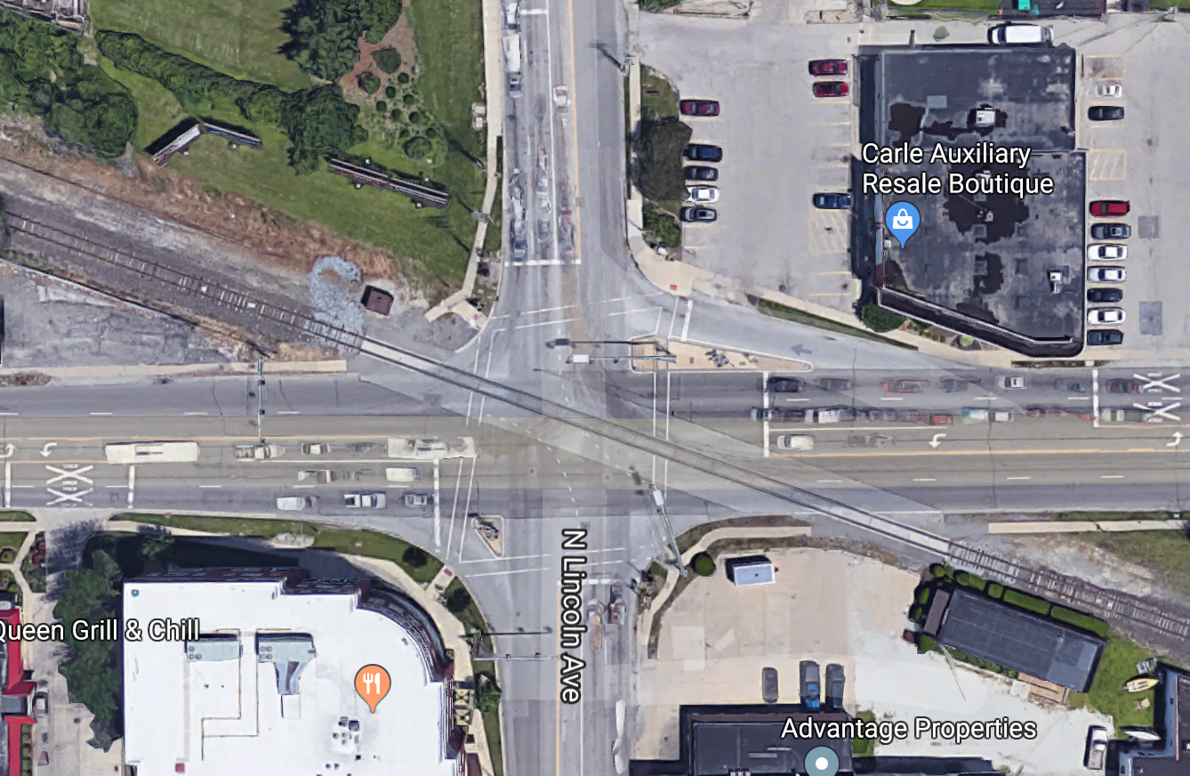
Some useful random variables might be:
| variable | domain (possible values) |
|---|---|
| time | {morning, afternoon, evening, night} |
| is-train | {yes, no} |
| traffic-light | {red, yellow, green} |
| barrier-arm | {up, down} |
Also exist continuous random variables, e.g. temperature (domain is all positive real numbers) or course-average (domain is [0-100]). We'll ignore those for now.
A state/event is represented by the values for all random variables that we care about.
P(variable = value) or P(A) where A is an event
What percentage of the time does [variable] occur with [value]? E.g. P(barrier-arm = up) = 0.95
P(X=v and Y=w)
How often do we see X=v and Y=w at the same time? E.g. P(barrier-arm=up, time=morning) would be the probability that we see a barrier arm in the up position in the morning.
P(v) or P(v,w)
The author hopes that the reader can guess what variables these values belong to. For example, in context, it may be obvious that P(morning,up) is shorthand for P(barrier-arm=up, time=morning).
Probability notation does a poor job of distinguishing variables and values. So it is very important to keep an eye on types of variable and values, as well as the general context of what an author is trying to say. A useful heuristic is that
A distribution is an assignment of probability values to all events of interest, e.g. all values for particular random variable or pair of random variables.
The key mathematical properities of a probability distribution can be derived from Kolmogorov's axioms of probability:
0 ≤ P(A)
P(True) = 1
P(A or B) = P(A) + P(B), if A and B are mutually exclusive events
It's easy to expand these three axioms into a more complete set of basic rules, e.g.
0 ≤ P(A) ≤ 1
P(True) = 1 and P(False) = 0
P(A or B) = P(A) + P(B) - P(A and B) [inclusion/exclusion, same as set theory]
If X has possible values p,q,r then P(X=p or X=q or X=r) = 1.
Probabilities can be estimated from direct observation of examples (e.g. large corpus of text data). Constraints on probabilities may also come from sceientific beliefs
Here's a model of two variables for the University/Goodwin intersection:
                             E/W light
                        green       yellow   red
 N/S light   green        0          0       0.2
             yellow       0          0       0.1
             red         0.5         0.1     0.1
To be a probability distribution, the numbers must add up to 1 (which they do in this example).
Most model-builders assume that probabilities aren't actually zero. That is, unobserved events do occur but they just happen so infrequently that we haven't yet observed one. So a more realistic model might be
                             E/W light
                        green         yellow     red
 N/S light   green        e            e         0.2-f
             yellow       e            e         0.1-f
             red         0.5-f       0.1-f       0.1-f
To make this a proper probability distribution, we need to set
f=(4/5)e so all the values add up to 1.
Suppose we are given a joint distribution like the one above, but we want to pay attention to only one variable. To get its distribution, we sum probabilities across all values of the other variable.
                             E/W light                marginals
                        green       yellow   red
 N/S light   green        0          0       0.2        0.2
             yellow       0          0       0.1        0.1
             red         0.5         0.1     0.1        0.7
-------------------------------------------------
marginals                0.5         0.1     0.4
So the marginal distribution of the N/S light is
P(green) = 0.2
P(yellow) = 0.1
P(red) = 0.7
To write this in formal notation suppose Y has values y1...yn. Then we compute the marginal probability P(X=x) using the formula P(X=x)=∑nk=1P(x,yk).
Suppose we know that the N/S light is red, what are the probabilities for the E/W light? Let's just extract that line of our joint distribution.
                             E/W light
                        green       yellow      red
 N/S light   red         0.5         0.1         0.1
So we have a distribution that looks like this:
P(E/W=green | N/S = red) = 0.5
P(E/W=yellow | N/S = red) = 0.1
P(E/W=red | N/S = red) = 0.1
Oops, these three probabilities don't sum to 1. So this isn't a legit probability distribution (see Kolmogorov's Axioms above). To make them sum to 1, divide each one by the sum they currently have (which is 0.6). This gives us
P(E/W=green | N/S = red) = 0.5/0.6 = 5/7
P(E/W=yellow | N/S = red) = 0.1/0.6 = 1/7
P(E/W=red | N/S = red) = 0.1/0.6 = 1/7
Conditional probability models how frequently we see each variable value in some context (e.g. how often is the barrier-arm down if it's nighttime). The conditional probability of A in a context C is defined to be
P(A | C) = P(A,C)/P(C)
Many other useful formulas can be derived from this definition plus the basic formulas given above. In particular, we can transform this definition into
P(A,C) = P(C) * P(A | C)
P(A,C) = P(A) * P(C | A)
These formulas extend to multiple inputs like this:
P(A,B,C) = P(A) * P(B | A) * P(C | A,B)
Two events A and B are independent iff
P(A,B) = P(A) * P(B)
It's equivalent to show that this equation is equivalent to each of the following equations:
P(A | B) = P(A)
P(B | A) = P(B)
Exercise for the reader: why are these three equations all equivalent? Hint: use definition of conditional probability. Figure this out for yourself, because it will help you become familiar with the definitions.
In lecture 9, I left the following question unanswered:
Near the end of AC-3, we push all arcs (C,X) onto the queue, but we don't push (Y,X). Why don't we need to push (Y,X)?
There's two cases. First (Y,X) might already be in the queue.
If neither of these situations holds, then we've already checked (Y,X) at some point in the past. That check ensured that every value in D(Y) had a matching value in D(X). And, moreover, nothing has happened to D(X) since then. So every value in D(Y) still has a matching value in D(X).
What we've just done in AC-3 is that D(Y) has become smaller. This means that some values in D(X) no longer have matching values in D(Y). But everything in D(Y) still has a matching value in D(X). This doesn't change when we remove unmatched values from D(X).
Autonomous drones seem an interesting idea to deliver packages. However, they have run into problems with the FAA and with angry residents. But the companies keep trying.