Gridworld pictures are from the U.C. Berkeley CS 188 materials (Pieter Abbeel and Dan Klein) except where noted.
Markov Decision problems and Reinforcement Learning are essentially one topic, with a series of graduate changes in assumptions and methods. The basic set-up is an agent (e.g. imagine a robot) moving around a world like the one shown below. Positions add or deduct points from your score. Its goal is to accumulate the most points.
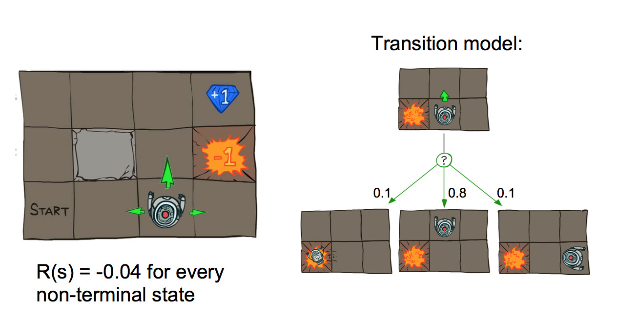
This could be a finite game but it's typically best to imagine a game that goes on forever. So ending or goal states reset the game back to the start.
Actions are executed with errors. So if our agent commands a forward motion, there's some chance that they will instead move sideways.
These methods can also be used for modelling board games but, most interestingly, learning how to control mechanical systems. For example, a long-standing reinforcement learning task is pole balancing.
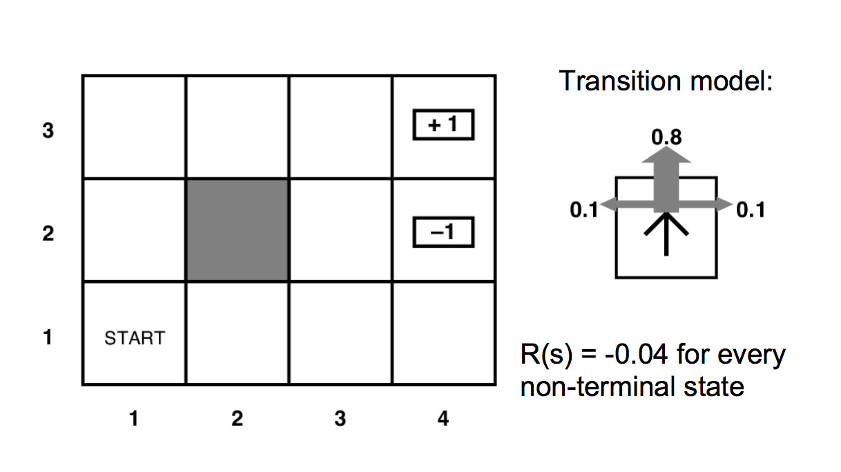
Eliminating the pretty details gives us a mathematician-friendly diagram:
Our MDP's specification contains
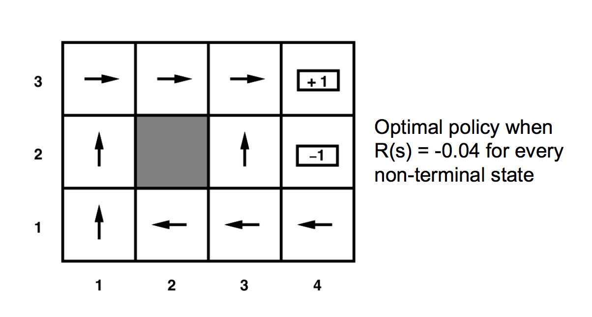
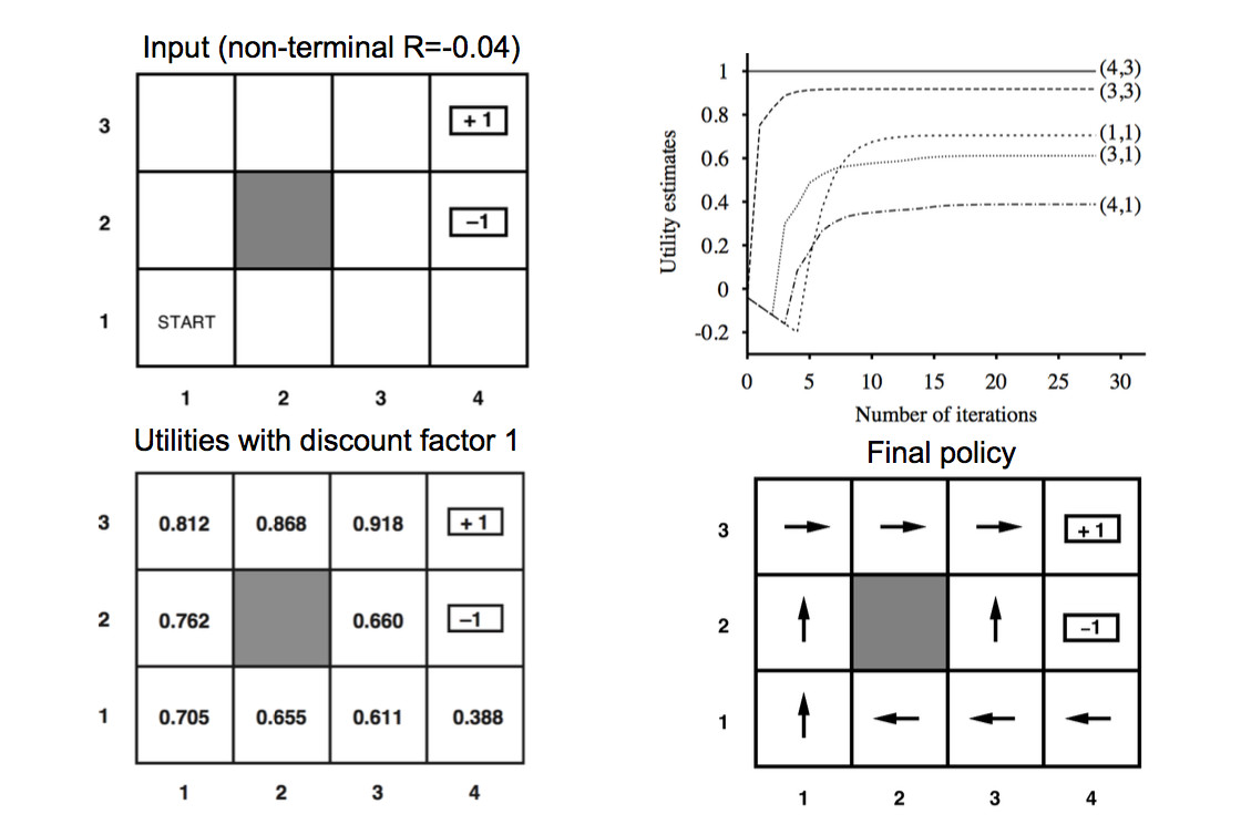
Our solution will be a policy \(\pi(s)\) which specifies which action to command when we are in each state. For our small example, the arrows in the diagram below show the optimal policy.
The reward function could have any pattern of negative and positive values. However, the intended pattern is
For our example above, the unmarked states have reward -0.04.
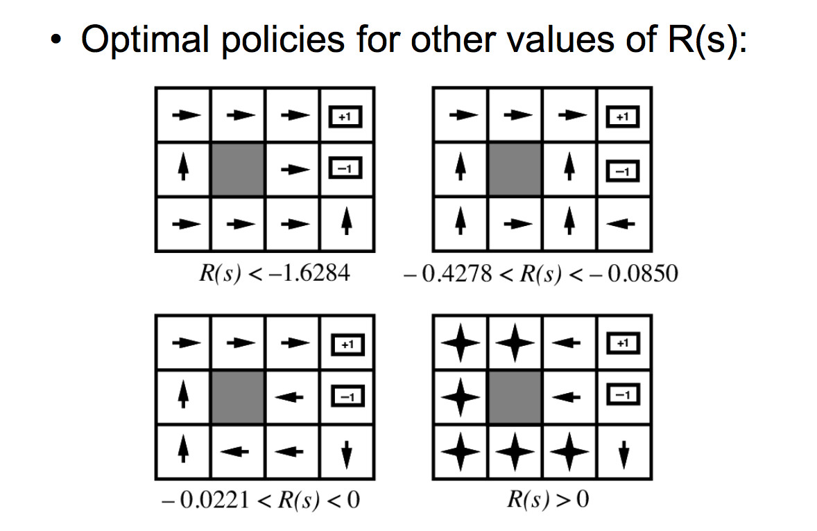
The background reward for the unmarked states changes the personality of the MDP. If the background reward is high (lower right below), the agent has no strong incentive to look for the high-reward states. If the background is strongly negative (upper left), the agent will head aggressively for the high-reward states, even at the risk of landing in the -1 location.
Want to maximize reward over time. So something like the sum of
P(sequence)U(sequence)
over all sequences of states.
U(sequence) is the utility of the sequence of states, i.e. the sum of the rewards. P(sequence) is how often this sequence of states happens.
Question: will the sums converge if I continue forever (mathematician) or a long time (engineer)?
A good way to think about the best policy is the "Bellman equation":relating the utility at each state s to the utilities at adjacent states:
\(U(s) = R(s) + \gamma \max_{a \in A} \sum_{s'\in S} P(s' | s,a)U(s') \)
The Bellman equation is recursive, so we'll have to figure out how to solve it. But just pretend that we already have utility values for each adjacent state s' and try to figure out how to use them to compute the utility of s.
Suppose that we command an action a. If we knew that we would end up in a particular state s', then this equation would give the utility for s in terms of the utility for s'. We pick the action a to maximize the output value.
\(U(s) = R(s) + \max_{a \in A} U(s') \)
Since our action does not, in fact, entirely control the next state s', we need to compute a sum that's weighted by the probability of each next state. The expected utility of the next state would be \(\sum_{s'\in S} P(s' | s,a)U(s') \), so this would give us a recursive equation
\(U(s) = R(s) + \max_{a \in A} \sum_{s'\in S} P(s' | s,a)U(s') \)
The actual Bellman equation includes a reward delay multiplier \(\gamma\). Downweighting the contribution of neighboring states by \(\gamma\) causes their rewards to be considered less important than the immediate reward R(s). It also causes the system of equations to converge.
Short version of why it converges. Since our MDP is finite, our rewards all have absolute value \( \le \) some bound M. If we repeatedly apply the Bellman equation to write out the utility of an extended sequence of actions, the kth action in the sequence will have a discounted reward \( \le \gamma^k M\). So the sum is a geometric series and thus converges if \( 0 \le \gamma < 1 \).
Suppose that we have picked some policy \( \pi \). Then the Bellman equation for this fixed policy is simpler because we know exactly what action we'll command:
\(U(s) = R(s) + \gamma \sum_{s'\in S} P(s' | s,\pi(s))U(s') \)
There's a variety of ways to solve MDP's and closely-related reinforcement learning problems:
The simplest solution method is value iteration. This method repeatedly applies the Bellman equation to update utility values for each state. Suppose \(U_k(s)\) is the utility value for state s in iteration k. Then
- initialize \(U_1(s) = \) for all states s
- loop for k = 1 until the values converge
- \(U_{k+1}(s) = R(s) + \gamma \max_{a \in A} \sum_{s'\in S} P(s' | s,a)U_k(s') \)
These slides show how the utility values change as the iteration progresses. The final output utilities and the corresponding policy are shown below.
You can play with a larger example in Andrej Karpathy's gridworld demo.