BFS & DFS
by Xin Tong, Zhenyi TangOverview
BFS and DFS are two simple but useful graph traversal algorithms. In this article, we will introduce how these two algorithms work and their properties.
BFS
The central idea of breath-first search is to search “wide” before search “deep” in a graph. In other words, BFS visits all the neighbors of a node before visiting the neighbors of neighbors. Because of this order of traversal, BFS can be used for finding a shortest path from an arbitrary node to a target node.
The queue data structure is used in the iterative implementation of BFS. The next node to process is always at the front of the queue and let’s call it . We dequeue from the queue, process it and enqueue all of its unvisited neighbors. Essentially, the queue ensures that nodes closer to the starting node will be visited earlier than nodes that are further away. The BFS traversal terminates when the queue becomes empty, i.e. all nodes have been enqueued into and later dequeued from the queue.
Pseudocode
BFSTraversal(start_node):
  visited := a set to store references to all visited nodes

  queue := a queue to store references to nodes we should visit later
  queue.enqueue(start_node)
  visited.add(start_node)

  while queue is not empty:
    current_node := queue.dequeue()

    process current_node
    # for example, print(current_node.value)

    for neighbor in current_node.neighbors:
      if neighbor is not in visited:
        queue.enqueue(neighbor)
        visited.add(neighbor)
Runtime Analysis
BFS runs in , where is the number of vertices and is the number of edges in the graph. This is because:
- Every node(vertex) is enqueued and processed exactly once, resulting in time.
- Every edge is checked exactly once when we do
for neighbor in current_node.neighbors, resulting in an additional time.
DFS
In contrast, depth-first search searches “deep” before it searches “wide”. If our current node has two neighbors n1 and n2 and we choose to visit n1 next, then all the nodes reachable from n1 will be visited before n2.
The stack data structure is used in the iterative implementation of DFS. The next node to process is always at the top of the stack and let’s call it . We pop from the stack and process it. Then one of ’s unvisited neighbors becomes the new if it exists. The DFS traversal terminates when the stack becomes empty, i.e. all nodes have been pushed onto and later popped from the stack.
Pseudocode
You can refer to the BFS pseudocode above. Just replace the queue with a stack and use stack methods!
Runtime Analysis
DFS runs in (same as BFS).
Traversal vs Search
BFS and DFS are suitable for both traversing the graph and searching for a target node. If the goal is to search, when we are at the target node, we can simply break out of the traversal routine and return that node or its value.
Comparison of Search Order
You can easily get an idea of the respective search orders of BFS and DFS from the figures below. We start BFS/DFS from the node circled in purple, and all nodes circled in yellow will be visited before nodes circled in red.
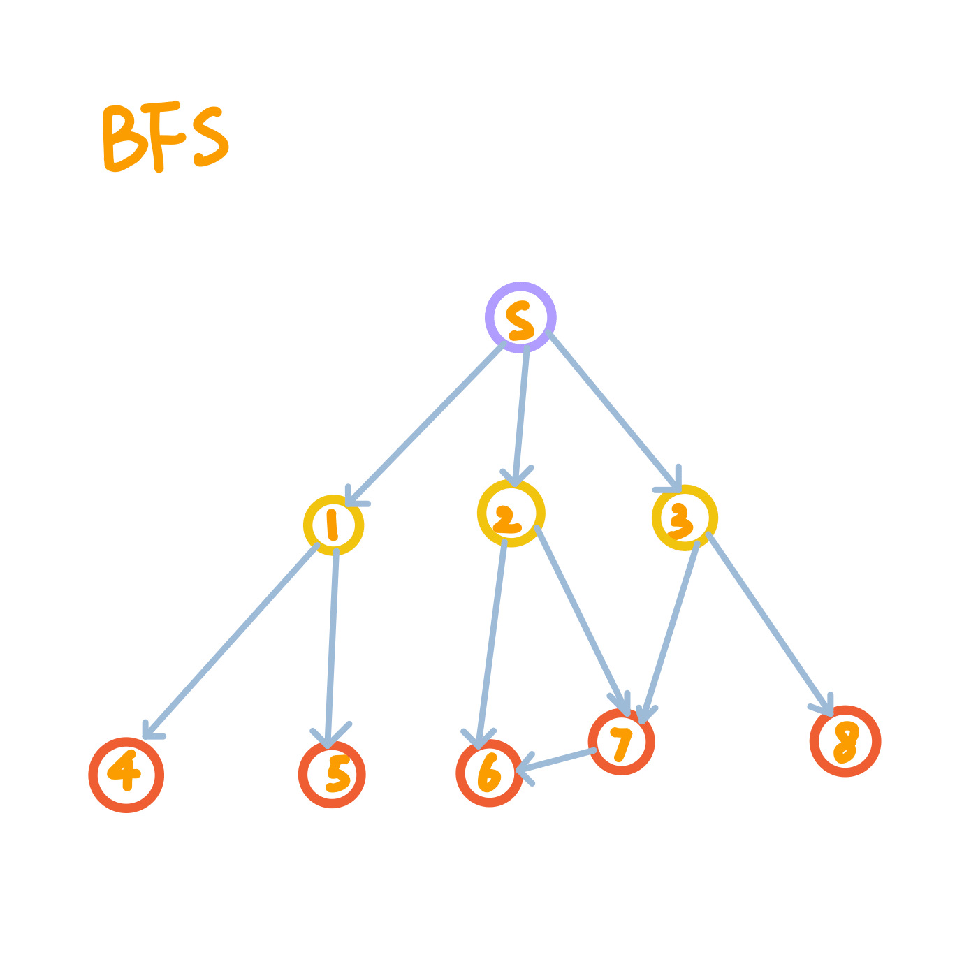
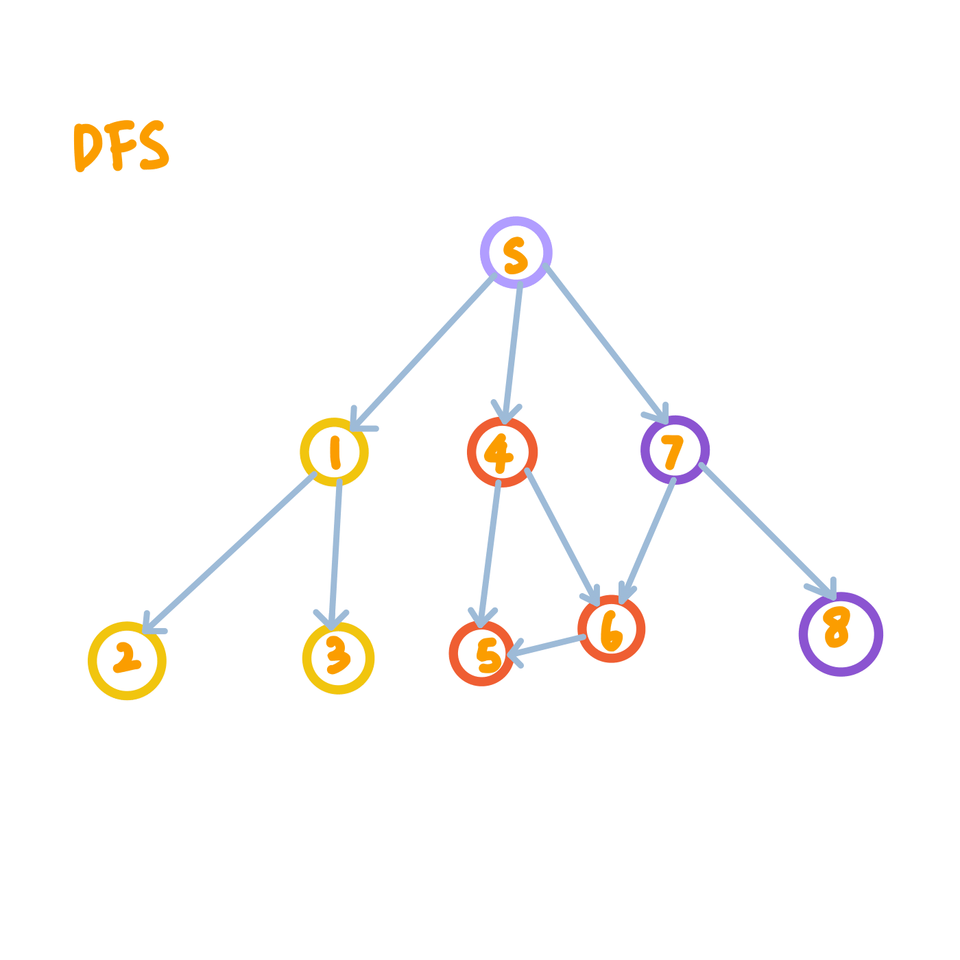
Note on Graph Properties
There are a few things to note about how BFS and DFS work on graphs with different properties:
-
BFS and DFS work on both directed and undirected graphs, as shown in the figures above.
-
If the underlying graph is disconnected, BFS and DFS can only traverse the connected component that the given starting node belongs to.
-
BFS cannot be used to find shortest paths on weighted graphs. See Dijkstra’s algorithm for that!