Lecture 13
Reading material: Chapter 7 of CSSB
Last lecture we introduced Laplace transform as a generalization of the Fourier Transform that is applicable to signals whose Fourier transform does not exist. In this lecture we spent a great deal of time learning about the Laplace transform of basic signals and how different mathematical operations can be translated to the Laplace domain. We will build a repertoire of common Laplace and time-domain pairs and then see how we can utilize that to solve both ordinary differential equations as well as initial value problems.
Basic Laplace transforms
In the last lecture we introduced the Laplace transform as a necessary generalization of the Fourier transform integral that is able to accommodate wider class of signals. We showed this by computing the Laplace transform of a hyperbolic sin for which the Fourier transform did not exist. However, there is far simpler and more ubiquitous signal whose Fourier transform doesn't exist but the Laplace transform does. This is the so called "on" signal or step signal (recall Lecture 04) defined as
However if the only advantage of defining the Laplace transform were to simply make some tough integrals converge its utility would have been offset by the loss in interpretability - i.e. we can interpret the Fourier transform as a change of basis for our time domain signals that exposes the underlying frequency contributions in its constitution. Alas no such easy to intuit explanation exists for the Laplace transform. Nevertheless, we have gained far more utility with this generalization as we will shortly see.
Mathematical operations & Laplace transforms
Consider the derivative of a function given as
where is used to denote the value of the signal at time . The negative sign is used to indicate that the negative time history of the signal up till has been lumped together into the value at . When the initial condition for the signal is zero (as is often the case) this extra term disappears.
Thus we get that as must be true of any generalization, the generalization must respect or uphold truths or results established by whatever mathematical object or concept was being generalized. The precise result being preserved here is the fact that the Laplace domain representation of the impulse function is still since . Indeed, recall that the derivative of the step function is the impulse function and thus we see that we can multiply with to get 1.
Now if differentiation in the time domain is represented in the Laplace domain as multiplication by then one can guess that the natural counterpart of differentiation being integration, the multiplication must be replaced by ... you guessed it: division! Isn't mathematics beautiful & orderly? In fact that particular bit of math works out to look like:
Therefore, in the presence of all zero initial conditions we can equate integration in time domain with division by in the Laplace domain - often called multiplication by for obvious reasons.
Solving convolutions
Another major result that we had when we learnt about Fourier analysis was the fact that convolutions in the time domain became multiplications in the frequency domain. Once again, as should be true of any generalization, this result remains unchanged in the Laplace domain. In other words
Example
Let us try to solve the following convolution using Laplace domain.
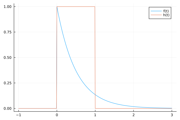
The functions in the above plot are as follows:
Then we have that
Therefore
Now to find the result we need to take the inverse Laplace transform of which we can do using Laplace transform tables if we can find the above functions in them. Often the tables of Laplace transforms will only have basic generic forms listed in them and the onus is on us to convert our functions into the forms given in the tables.
One particular technique that is useful here is to be able to break apart complex fractions like the above into their constituents. This is called the technique of partial fractions which is a powerful and very useful one to have under our repertoire. Here we will show the technique in action for now but relegate the general treatment to the next section.
Consider:
Taking the inverse Laplace transform gives:
which we plot below along with the original functions. 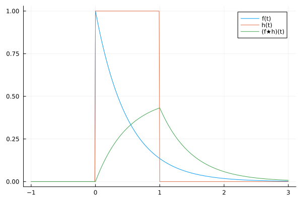
Now we turn our attention to the general procedure for finding partial fraction expansions (PFE).
General method of partial fractions
The basic objective in the method of partial fractions is to decompose a proper rational fraction (a rational fraction is proper only if the degree of the numerator is lower than the degree of the denominator) into simpler constituents. Here is the general strategy:
Start with a proper rational fraction. If improper, then perform polynomial long division first and focus on the part that is proper.
Factor the denominator into linear and irreducible higher order terms. A term or factor is called irreducible if it cannot be factored further using rational numbers: e.g. is irreducible because factoring it requires writing:
which involves an irrational: .Next, write out a sum of partial fractions for each factor (and every exponent of each factor) using the forms/rules for PFEs (see table below).
Multiply the whole equation by the bottom/denominator and solve for the coefficients.
The form of the partial fraction written in Step 3 depends on the form of the factor in the denominator as elucidated in the following table:
| Type | Partial Fraction Decomposition |
|---|---|
| Non-repeated linear factor | |
| Repeated linear factor | |
| Non-repeated quadratic factor | |
| Repeated quadratic factor |
As you can see, when we have a repeated factor we have to write a partial fraction for it as many times as it repeats (with different powers as well). We now do an example to illustrate the above steps.
Partial fractions example:
Find the partial fraction decomposition of:
Solution: Fortunately the denominator is already factored for us and consists of two repeated linear terms and a non-repeated linear term. So we have:
For example gives us because:
Similarly, one can (and you should) verify that gives us that .
Using the values of and with gives us that (again verify this).
Thus,
Now it may not always be the case that the method of partial fractions will be solvable by trying different values of as in (2). Sometimes we may need to set up a system of linear equations to solve for the coefficients or resort to using software. Below follows an example where this happens:
Example redux
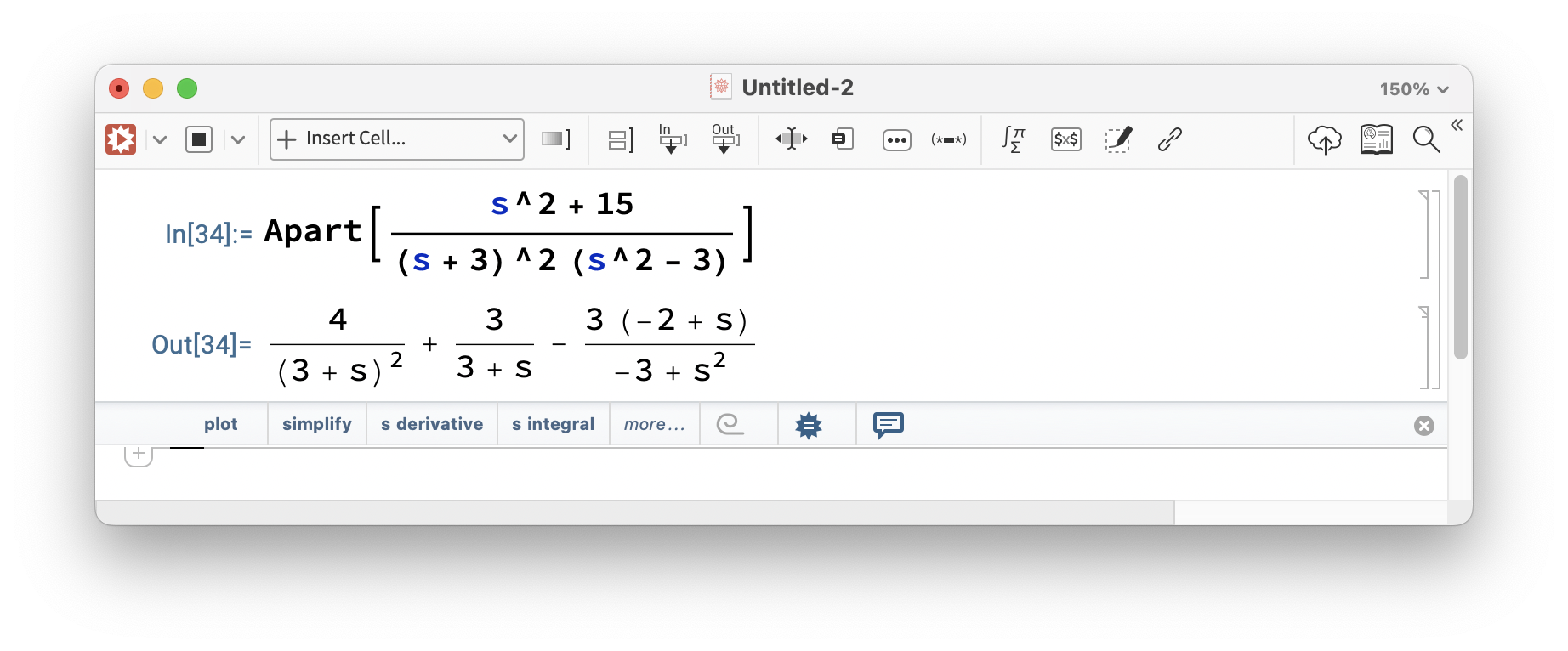
Find the partial fraction expansion of:
Solution: Again the denominator is already factored for us and consists of a twice repeated linear terms and a single quadratic term (why?). Therefore as per the table above we get that:
But that is pretty much the only headway we can make here to get at the uppercase coefficients directly. What we will need to do next is to substitute in this value of into the above equations and collect like powers of to compare coefficients. This will give us a linear system of three equations in three unknowns. One can verify that these are:
Partial fractions in software
Fortunately, we can use MATLAB (or some other software package) to solve partial fraction problems[1]. In this section we will show examples of using software to solve the above problems. As usual with software toolkits, using the right tool for the correct job makes life easier.
The most straightforward method is to use a CAS. For example Mathematica implements this as Apart.
but our go-to software in this course is either MATLAB or Python so we look at MATLAB next. In MATLAB the command we will use is called residue and the code snippet below shows how we solve the first problem above.
clear
numerator = [3, 1];
denominator1 = fold(@conv, {[2,-1],[1,2],[1, 2]});
[num, roots, const] = residue(numerator, denominator1)

% If the fold function does not work then that single line above
% is equivalent to the following:

den_factors = {[2,-1],[1,2],[1, 2]};
denominator2 = [1];
for i=1:length(den_factors)
    denominator2 = conv(denominator2, den_factors{i});
end
which gives
num =

   -0.2000
    1.0000
    0.2000

roots =

   -2.0000
   -2.0000
    0.5000

const =

     []
The output suggests that the partial fraction expansion is:
A similar exercise in coding shows that the second example from above can be formulated as follows:
clear
numerator = [1, 0, 15];
denominator = fold(@conv, {[1,0,-3],[1,3],[1, 3]});
[num, roots, const] = residue(numerator, denominator)
with output:
num =

    3.0000
    4.0000
    0.2321
   -3.2321

roots =

   -3.0000
   -3.0000
    1.7321
   -1.7321

const =

     []
But here we run into trouble because MATLAB factored the term further using (see footnote 1).
One (particularly unsatisfactory) way around this limitation is to use the partfrac from MATLAB's Symbolic Toolbox (which might involve paying for yet another add-on to MATLAB):
syms s
partfrac((s^2+15)/((s+3)^2*(s^2-3)))
The above gives:
ans = 3/(s+3) - (3*s-6)/(s^2-3) + 4/(s+3)^2
Things are a bit simpler in Python (for those of you interested) but requires the use of the SymPy package
from sympy import symbols, apart

s = symbols('s')
numerator = s**2+15
denominator = ((s+3)**2)*(s**2-3)
frac = numerator / denominator
print(apart(frac))
which results in:
-3*(s - 2)/(s**2 - 3) + 3/(s + 3) + 4/(s + 3)**2
Solving ODE's in the presence of nonzero initial conditions
As remarked previously, the one-sided Laplace transform (when properly taken) ends up having a term (see Eq. (1) for example). In the following we will make use of this to see how we can solve initial value problems. Consider a mass-spring and damper system from our in-class lectures:
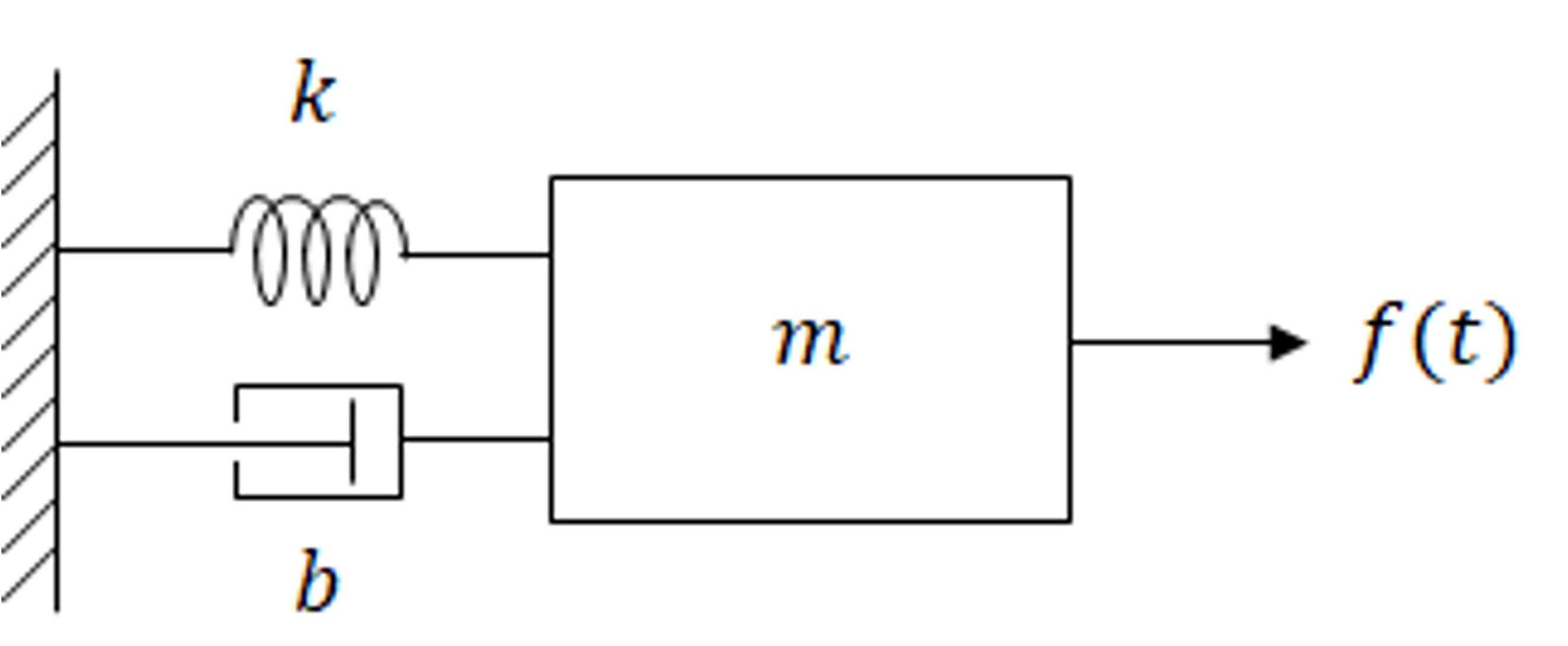
We have derived that the dynamical equations for such a system are:
where is the displacement of the mass from its equilibrium position, is the spring constant, is the damper coefficient and is the mass in kilos of the attachment. Here is the forcing function or input into the system. Then if we take the Laplace transform of (6) above we get:
In (7) above we have used the following fact (stated without proof but alluded to above):
Theorem: (Higher derivatives in Laplace domain)
Suppose that , , are all continuous functions whose Laplace transforms exist.
Then:
Now consider the two cases:
Zero initial conditions
If the mass was at rest in its equilibrium position then we have . Suppose for simplicity kg and Ns/m and N/m. Thus (7) above reduces to:
which looks like:
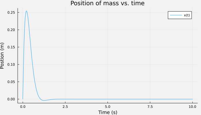
Does the plot make sense?
A 1 kilo mass was attached to a spring that requires 25N to compress it 1 meter and a damper that produces 8N of force of if you try to move it at 1m/s speed. Then this system was hit with a force equal to three times the standard impulse. While it moved, the relatively strong damping and spring meant it didn't move much and returned quickly to equilibrium.
Non-zero initial conditions
Suppose instead the mass was displaced units from its equilibrium position and released at time with velocity m/s. This means and . Then (7) above becomes:
If you plot the answer it should look like this:
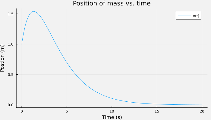
Does the plot make sense?
The plot starts at so the initial condition was respected. The mass had an initial displacement of units and also was released with an initial velocity m/s (hence in same direction as the displacement). So ... it actually ends up moving away from its equilibrium position (of ) initially until the spring starts pulling it back. The relatively heavy damping then smoothly (but also slowly) brings it to rest at in about 20 seconds.
Clearly from the plots above, the values of damping coefficient in second order systems has a huge effect on the solution profiles. We will investigate this in depth in the next lecture.
| [1] | ... with a few caveats. More specifically, the answer MATLAB gives you may not always be the answer you want. |