Lecture 12

Reading material: Chapter 6 of CSSB

Last lecture, we spent a considerable amount of time discussing the frequency response of a system, the meaning of the system spectrum, analytically computing the system response to sinusoid inputs, simple block diagram algebra, etc. We ended the lecture discussing a systematic way to draw magnitude & phase diagrams given a system transfer function using the Bode plot technique. We continue this thread in this lecture.

Block diagram algebra

We discussed in class some basic rules of block diagram manipulation and algebra. These notes are available here and class is expected to be familiar with the techniques discussed therein and should have been useful for completing homework assignments as well.

Bode plot examples

Let us consider a few examples of plotting Bode diagrams (i.e. the magnitude/phase plots) for a few system transfer functions. To review what the plots of Bode primitives look like check out this interactive demo.

Example 1

Let us start with the example we considered in the last lecture. Namely,

$$G(s) = \frac{s+3}{s(s^2 + 2s + 4)}$$

Recall that in Bode form it had was written as:

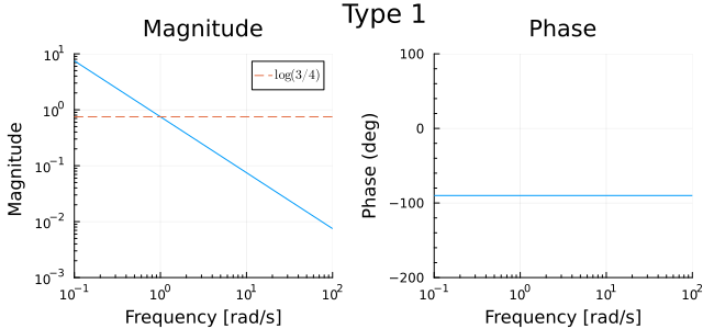
Type 1 factor

The Type 1 factor here is $3/4 \left(j \omega \right) ^{-1}$. It has a negative unity exponent and $K=3/4$. We already showed in the previous lecture what the Type 1 factor for this transfer function will contribute to the Bode plot. These figures are reproduced here for consistency.

Type 2 factor

For the Type 2 factor in this transfer function, that is,

we see that it has a positive unity as exponent and $\tau = 1/3$. Thus the magnitude and phase plot for this term are as follows:

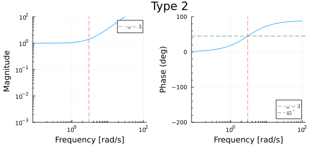
The magnitude plot is horizontal until near the breakpoint and then proceeds upwards with slope 1 while the phase plot climbs from $0$ to $90^\circ$ by hitting $45^\circ$ at the breakpoint.

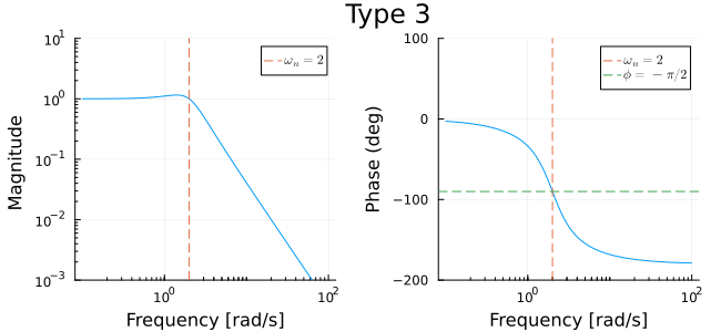
Type 3 factor

The type 3 factor in this case is

which has negative unity as exponent, $\omega_n = 2$ and $\zeta = \dfrac{1}{2}$. Therefore for the magnitude plot, the graph is horizontal until it reaches near the natural frequency whereupon it descends downwards with slope 2. Similarly the phase plot goes from 0 to $-180 ^\circ$ passing through $-90 ^\circ$ at the natural frequency.

Combining plots

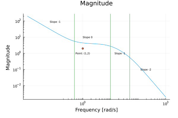
The final plot is a pointwise addition of all the graphs above. For example we know the phase plot will start at $-90 = -90 + 0 + 0$ where the terms on the right of the equality are contributions from the Type 1, Type 2 and Type 3 factors. Similarly, we know it will end at $-180 = -90 + 90 -180$. If the breakpoint frequency $1/\tau$ of the Type 2 term and the natural frequency $\omega_n$ of the Type 3 term where the same, we could have expected the phase plot to cross $-135^\circ = -90^\circ +45^\circ -90^\circ$ at this joint frequency. However, $\omega_n < 1/\tau$ and so the phase plot crosses $-135^\circ$ much earlier.

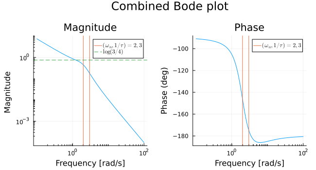
In the same way we can reason about the magnitude plot. We know it will start out with a slope of negative unity. But once the frequency passes beyond the breakpoint/natural frequency, the Type 2 term will add a slope of positive unity; at the same time the Type 3 term will contribute $-2$ to the slope. So the slope of the graph beyond the breakpoint will be $-1 + 1 - 2 = -2$. Therefore the overall plot is two segments of slope -1 and -2 joined around the the breakpoint/natural frequency with a small kink.

Example 2

Consider the following transfer function:

$$G(s) = \dfrac{2000\left(s + 0.5\right)}{s \left(s+10\right)\left(s+50\right)}$$ Exercise: Convert (2) to Bode form:

This function has one factor of Type 1 and three factors of Type 2.

Type 1 term

This term is $\dfrac{2}{j \omega}$. Here $K=2$ and $n=-1$. This factor contributes a line of slope $-1$ passing through $(\omega, M) = (1, 2)$. Since $n=-1$ its phase plot starts at $-90^\circ$.

Type 2 terms

These terms are:

with $\tau_a = 2, \tau_b = 1/10$ and $\tau_c = 1/50$. We can consider their contributions to the magnitude plots as follows:

• The magnitude plot will start with a slope of -1.

• When $\omega = 0.5$, the first Type 2 factor contributes a slope increase of 1.

• When $\omega = 10$, the second Type 2 factor contributes a slope decrease of 1.

• When $\omega = 50$, the third Type 2 factor again contributes a slope decrease of 1.

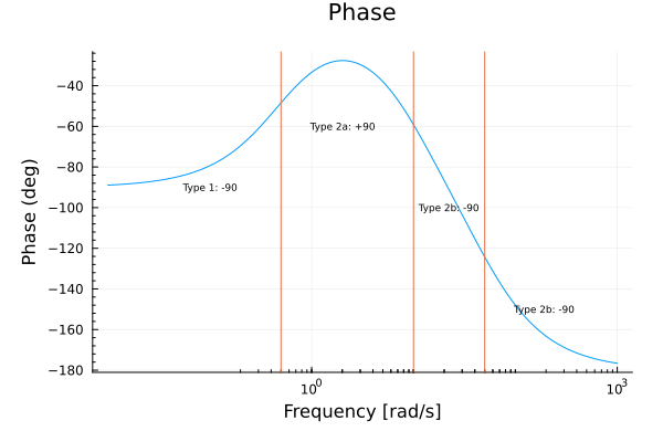
We can similarly reason about the phase plots:

• From the Type 1 factor we know the graph will start at $-90^\circ$.

• At $\omega =0.5$, the first Type 2 term adds a phase contribution of $90^\circ$.

• At $\omega=10$, the second Type 2 factor adds a phase of $-90^\circ$.

• At $\omega=50$, the third Type 2 factor adds yet another contribution of $-90^\circ$.

• Together, this means the phase plot ends at $-180^\circ$.

Example 3

Consider the following transfer function which is already in Bode form:

$$G(s) = \dfrac{0.01 \left(s^2 + 0.01s + 1\right)}{s^2 \left(\dfrac{s^2}{64} + 0.02 \dfrac{s}{8} + 1 \right)}.$$

This transfer function has a single Type 1 factor and two Type 3 factors.

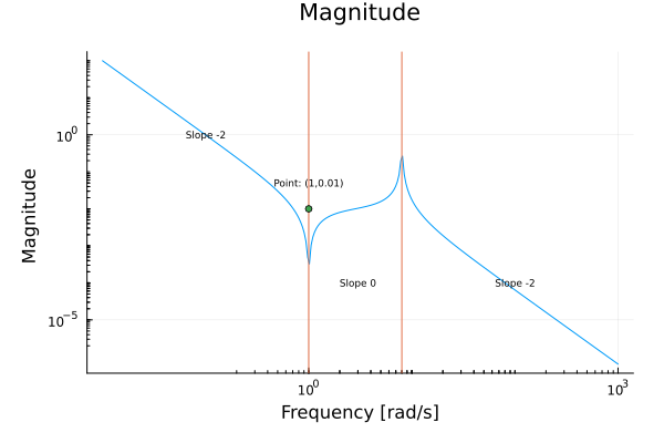
For its magnitude plot we have that,

• The Type 1 factor with $K=0.01$ and $n=-2$ contributes a line of slope -2 passing through the point $(\omega, M) = (1, 0.01)$.

• The Type 3 factor with positive exponent has natural frequency $\omega_n=1$ and damping coefficient $\zeta=0.005$. It contributes a slope increase of 2 beyond $\omega =\omega_n$ along with a resonance dip.

• The Type 3 factor with negative exponent has natural frequency $\omega_n=8$ and $\zeta=0.01$. It contributes a slope decrease of 2 beyond $\omega = \omega_n$ along with a resonance peak.

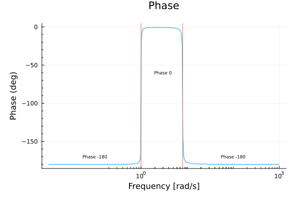
For its phase plot we have that,

• The Type 1 factor has exponent negative 2, therefore the phase plot starts at $-2 \times 90 ^\circ = 180^\circ$.

• At $\omega_n = 1$ the first Type 3 factor contributes a phase increase of $180^\circ$.

• At $\omega_n = 8$ the second Type 3 factor contributes a phase decrease of $180 ^\circ$.

• Since $\zeta$ is very small for, both Type 3 factors have sharp transitions (see demo).

Bode plots using software

One can solve for the above examples in MATLAB using the following code.

Example 1 - MATLAB

In this example we make use of the Control System Toolbox in MATLAB while in the next example we will make plots without relying on the toolbox. Recall that the transfer function (1) is:

The below code generates the final Bode plot.

num=[1, 3];         % Numerator coefficients
den=[1, 2, 4, 0];   % Denominator coefficients
sys = tf(num, den); % Transfer function model
bodeplot(sys);      % Generate bodeplot
title("Final Bode Plot - Example 1")
grid on;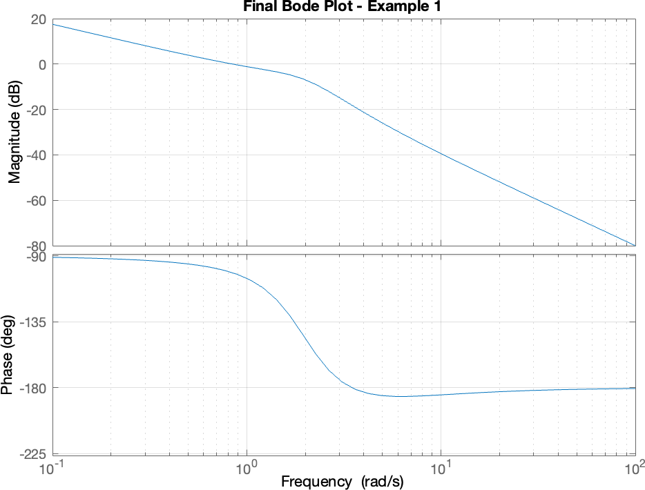

The below code also shows the term by term contributions.

typ1 = tf(3,[4, 0]);		%TF from just Type 1 term
typ2 = tf([1/3, 1], 1);		%TF from just Type 2 term
typ3 = tf(1, [1/4, 1/2, 1]); 	%TF from just Type 3 term

bodeplot(typ1);
hold on
bodeplot(typ2);
bodeplot(typ3);
legend('Type 1', 'Type 2', 'Type 3')

Exercise: Solve this problem in MATLAB without using the Control Systems Toolbox.

Example 2 - MATLAB

In this example (i.e. transfer function of (2)),

we generate the magnitude/phase plots without using any toolboxes.

den = @(w) (w.*j).*(w.*j+10).*(w.*j+50);
num = @(w) 2000.*(w.*j + 0.5);
tf = @(w) num(w)./den(w);


w = logspace(-2,3, 1000);
subplot(1, 2, 1)
loglog(w, abs(tf(w)));
xlabel("Frequency [rad/s]")
ylabel("Magnitude")
title("Magnitude plot")
grid on

subplot(1, 2, 2)
semilogx(w, angle(tf(w))*180/pi);
grid on
xlabel("Frequency [rad/s]")
ylabel("Phase angle")
title("Phase plot")
sgtitle("Magnitude/phase plot for Example 2 above")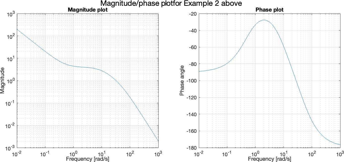

Example 3 - MATLAB

Left as an exercise. Plot in MATLAB the transfer function of (3).

Introduction to the Laplace transform

So far we have had a great run, so this now is as good a place as any to take stock of how far we have come:

• we started the semester by defining what signals are for our purposes

• we have learned to manipulate signals mathematically

• we have explored in depth the most basic of signals (i.e. sinusoids)

• we have become capable of decomposing a vast class of signals into these basic constituents (i.e. transformation to frequency domain)

• we have developed skills necessary to make deeper characterization of signals using their frequency domain representations

• along the way, we picked up a plethora of statistical concepts and techniques including correlations, orthogonality, etc.

• next we extended our tools to not just analyze signals, but also systems that act on signals

• for a large class of systems (i.e. LTI systems) we can now compute how they respond to arbitrary inputs by studying their transfer functions

Having accomplished this much, it is pertinent to ask how extensible and generic are the techniques we have developed?

Omission #1

Admittedly we glossed over a few (possibly important) details in our treatment of systems so far. Consider the two systems below:

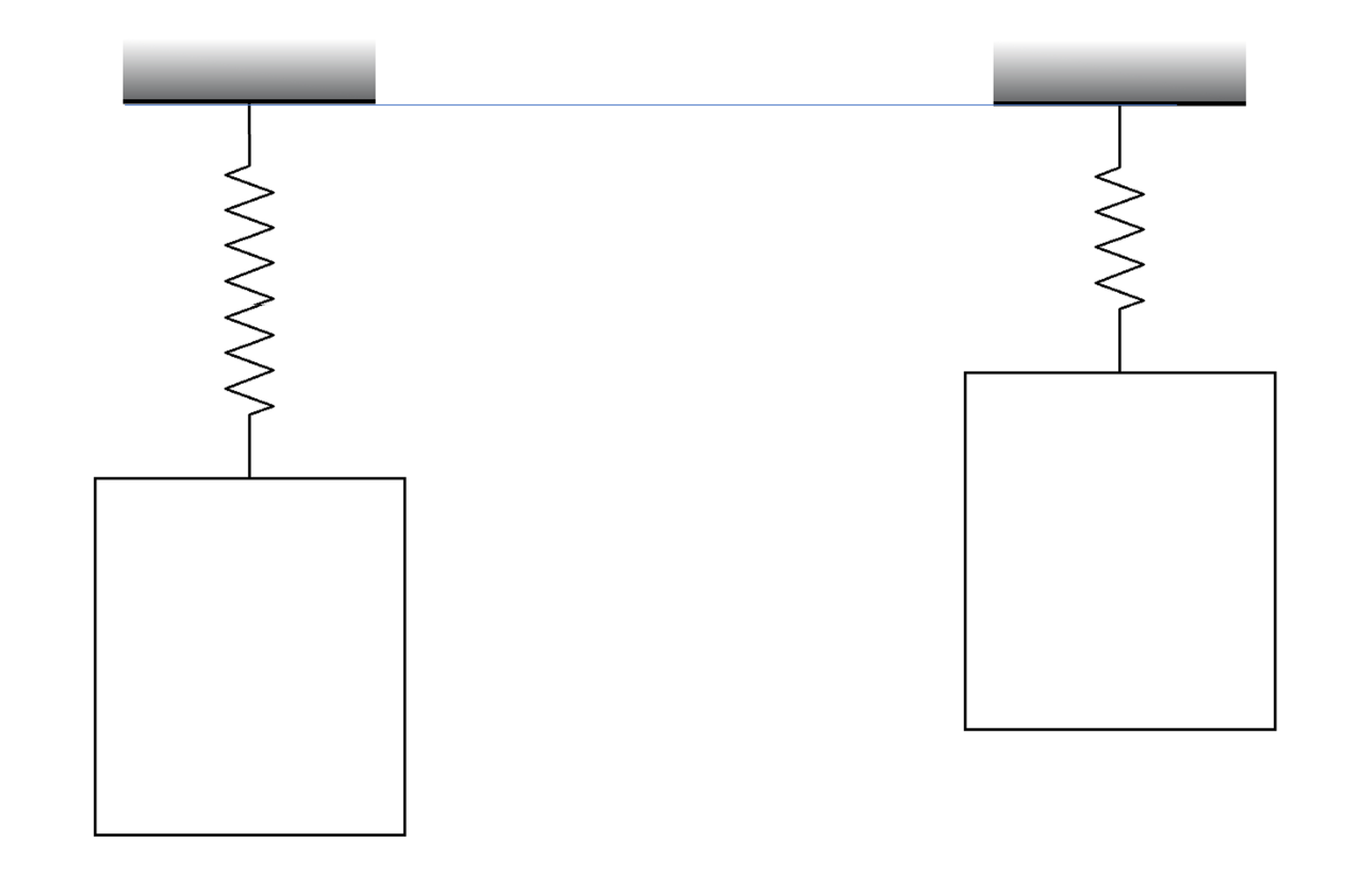
On the left we have a mass-spring system where the spring is in its elongated state whereas on the right we have the same system where the spring is in its equilibrium state.

Question: If at time $t>0$, the same input $x(t)$ was applied identically to both systems, are their responses going to be identical?

Thus, one glaring omission/fault in our treatment of system responses so far has been the neglect of initial conditions and its effect on the system response^[1]. More precisely speaking, in all our treatments so far, we have implicitly assumed that all the initial conditions are zero.

Omission #2

Arguably, one of the great advantages or benefits we derived from ploughing through all the math regarding Fourier analysis is the ability to turn a complicated integration in the time domain to a simple multiplication in the frequency domain. In more mathematical terms, we transformed an integral operation on one hand to an algebraic manipulation on the other - provided that we are able to take the Fourier transform. This naturally begs the question:

Question: Are there signals whose Fourier transform does not exist?

Enter the Laplace transform

The (classical) Fourier transform can be seen as a special case of the Laplace transform which attempts to fix the above issues. First off, as must be true of a generalization, there are some functions that do not have a (classical) Fourier transform representation that do have a Laplace transform representation. So, we can use the Laplace transform to handle those functions that the Fourier transform cannot. Second, the Laplace transform, naturally admits a way to incorporate nonzero initial conditions when solving for system responses ^[3].

The central idea behind the generalization (at least for the purposes of this class) is this: interpret the Fourier transform integral

$$F(\omega) = \int \limits _{-\infty} ^{\infty} f(t) e^{-i\omega t} dt$$

as evaluating the integral of a function multiplied by a complex exponential where $\omega$ is only allowed to move along the imaginary axis of the complex plane. The key generalization is to relax this restriction and to allow the complex exponential to take value off the imaginary axis as well:

where the intuition is $e^{-st} = e^{-\sigma t} e^{-i\omega t}$ and the $e^{-\sigma t}$ is fast decaying exponential for large enough $\sigma >0$ and will make most functions $f(t)$ go to zero so the integral will converge. Thus we get the definition of the bilateral (or two-sided) Laplace transform as:

This integral is supposed to be understood in the sense of an improper integral that only converges if each of the pieces

themselves converge. More importantly for us, the above is not the definition of the Laplace transform we will use; rather we will mostly concern ourselves, with the unilateral (or one-sided) Laplace transform:

$$\mathcal{L}\left[f(t)\right] := \int \limits _{0} ^{\infty} f(t) e^{-st} dt$$

The precise technical reasons for this choice is beyond the scope of these notes; but the short & sloppy version is to recall we deal with causal systems, i.e. cause (stimulus) precedes effect (response) and so the more appropriate integral^[4] is the one that starts at $t\ge 0$. It is also precisely this choice that will allow us to readily encode the initial value, i.e. value at $t=0$ into our analysis framework as we will see in later lectures. We end this one with a straightforward computation showing that the Laplace transform of the hyperbolic sine exists (above we showed it didn't work for the Fourier transform). We have:

where in the above we have used the fact that the Laplace transform $\mathcal{L}\left( e^{at} \right)$ is $\dfrac{1}{s-a}$. We leave it as an exercise to prove this fact.

Exercise: Show that the Laplace transform of $e^{at}$ is

$$\mathcal{L}\left( e^{at} \right) = \dfrac{1}{s-a}$$

[back]

[1]	The astute reader will note that this neglect did rear its head before once; see note at the bottom of this section vis-a-vis convolution and FFT. Specifically, the FFT method only gave the steady state response!

[2]	A more traditional approach is to consider the Fourier transform of $e^{at}$ where $a>0$; however in this case while the Fourier transform does not exist in the usual sense of functions, one can concoct an answer in terms of the Dirac delta and distributions (i.e. generalized functions).

[3]	Technically, we could do this with the Fourier approach as well, but it the payoff for the effort is negligible compared to the versatility we get by simply using the Laplace transform.

[4]	Why didn't this apply to the Fourier transform? Again, beyond the scope - but recall that was predicated on periodic functions which repeated indefinitely in either direction of the time axis.