In the last lecture we discussed convolutions, impulse response of LTI systems, the relationship between the impulse response of LTI systems and convolutions, the relationship between multiplication in the frequency domain and convolutions in the time domain. We further saw code examples on how to compute the system response to a given input if we know the impulse response. In this lecture, we continue our study of systems concepts; specifically we will study the concepts of frequency response, systems spectrum, transfer functions and system diagrams.
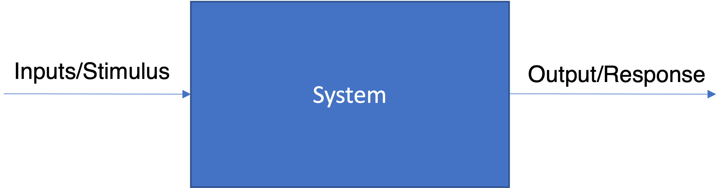
Recall from from the very first lecture that we have a graphical method of representing systems and signals called system diagrams as shown below.
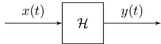
Now that we know about the impulse response of a system, in the following we will represent systems with the letters H,G,P as appropriate and generally use x(t) and y(t) to represent the input and output to systems.
We call the process by which a system H transforms the input x(t) to the output y(t) the action of H on x(t). More colloquially, y(t) is produced by Hacting on x(t). We represent this mathematically as y(t)=H(x(t))). Often for ease of notation, we drop the argument t when it is understood the signals x and y are functions of time: y=H(x).
Often it is quite useful to break down a complex system into its constituent elements or conversely, to build up a complicated system behavior by the composition of simpler constituent elements. There are two basic ways of composing systems as outlined below.
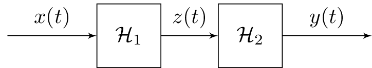
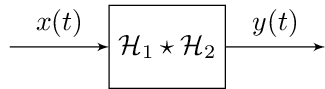
Borrowing terminology from circuit analysis, the first method of composing two systems is called a series connection. In such a composition, the output of one system element is fed in as input to the second system element.
The output y(t) in such a case can be represented as y=H2(H1(x)).
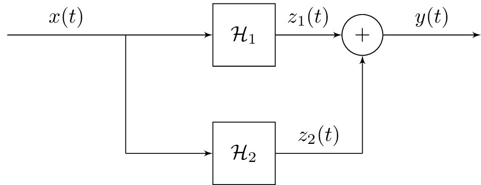
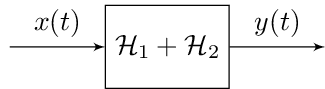
The second way of composing two system elements is to connect them in parallel as shown below.
The summation element (shown by a circle above) is a new feature in our systems diagram. In the parallel connection above, the input is fed separately to two subsystems and their outputs are summed together to produce the final response: y=H1(x)+H2(x).
For LTI systems we know the output y(t) to an in input x(t) can be written in terms of the impulse response h(t) as y(t)=h(t)⋆x(t). Thus the above interconnections simplify. Indeed for the series connection we have the output ys is:
ys=h2⋆z=h2⋆(h1⋆x)=(h2⋆h1)⋆x
Similarly for the parallel connection we have that the output is:
yp=z1+z2=(h1⋆x)+(h2⋆x)=(h1+h2)⋆x
Therefore the LTI series interconnection of two systems with impulse responses h1 and h2 results in a system with overall impulse function: h1⋆h2 and the parallel interconnection results in a system with overall impulse function h1+h2.
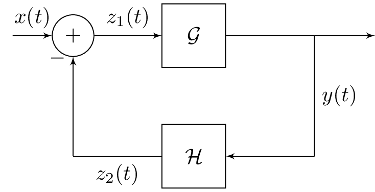
Recall that we discussed the use of feedback to desirably modify the process or characteristics of a system when we talked about different approaches to modeling biological systems. We are now in a position to analyze with tools at our disposal the feedback interconnection diagram. Consider the feedback interconnection diagram given below:
Then we have the following relations:
z2=y⋆H
z1=x−z2
y=z1⋆G
Starting with the last equation we have that:
y=z1⋆G=(x−z2)⋆G=(x−y⋆H)⋆G=x⋆G−y⋆H⋆G
which we can rearrange to get
y⋆(δ+G⋆H)=x⋆G
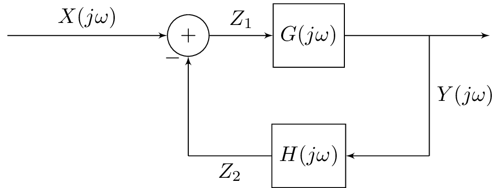
The above equation can and is often presented in a much cleaner format by switching representations to the frequency domain. Indeed then, the above diagram becomes:
and we get:
XY=1+GHG
which is very important equation that we can use to simplify algebraically many interconnections between system elements as we will see in the examples below. The ratio in (1), the ratio of the output to the input in the frequency domain, is an important enough quantity that it gets its own name: transfer function. We will spend entire lectures talking about transfer functions, and so now is as good a time as any to understand its definition - the frequency domain[1] ratio of the output to the input.
The same quantity as in (1), that is the ratio of the output to the input is a very general abstraction that applies to a large class of systems. However, when specialized to simple LTI systems, it has a nom de guerre; specifically, it is called the frequency response. To see why this is an apt name, it is instructive to examine the response of an LTI system with impulse response h(t) to a (complex) sinusoidal input x(t)=ejωt. We have that:
Thus we have that the output from the system is still a complex exponential (or sinusoid) with the same frequency but now modulated by a H(jω) factor in front of it.
Key point: Therefore we have that any stable LTI system with zero initial conditions responds (in steady state) to sinusoidal inputs with sinusoidal output of the same frequency; albeit with changes in amplitude and phase.
How the input sinusoids amplitude and phase are changed is a function of the complex frequencyjω, as defined by the frequency responseH(jω).
⚠️ Note
The qualifier - "in steady state" - is required because as shown in a class activity, there can be transient portions in the system response which fade away with time. Similarly, we will deal with nonzero initial conditions when we introduce the Laplace transform and stability of a system is a topic for later lectures.
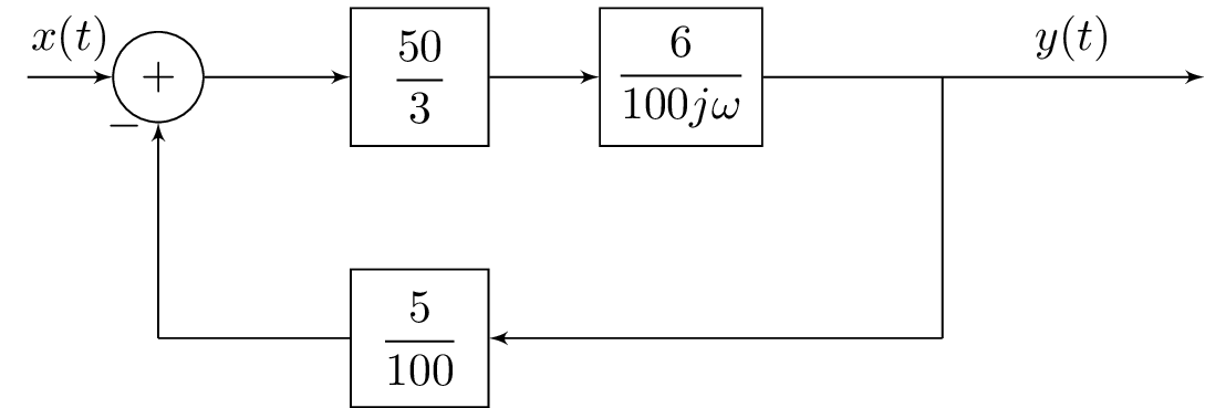
Consider the system below with a sinusoidal input x(t)=0.6sin(0.3t+20). What is the system response?
Solution: To use the result of Example 1 above let us convert the input to a cosine: x(t)=0.6cos(0.3t−70). Application of (1) with the observation made for LTI series connection results in the overall transfer function given as
H(jω)=−20ω+j20j
We can compute the magnitude and phase of H(jω) as a function of ω. Indeed,
M(ω)=400ω2+120andφ(ω)=π/2−arg(j−20ω)
Plugging in ω=0.3 we get M(3/10)=20/37. Similarly, φ(3/10)=arctan(1/6)−π/2≈−80.5∘. Thus we get that the output response should be:
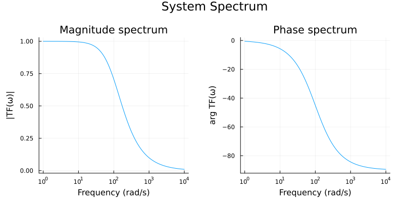
While the spectrum of a signal tells us the how energy in a signal is distributed amongst the constituent frequencies in the signal, the spectrum of a system tells us how the system modifies an input signal - both by amplifying or attenuating its amplitude as well by modifying the phase characteristics. Thus, the magnitude spectrum of a system looks very much like the magnitude/phase spectrum plots we have seen so far. The below figure shows the spectrum of hypothetical system.
We can see that the system characterized by the above spectrum is a low pass filter with a cutoff frequency of 100 Hz. How do we know 100 Hz is the cutoff frequency? Recall that the cutoff frequency is where you get half power. In the above figure, the magnitude plot has no units (not in decibel scale). Since power directly related to amplitude squared, we would get half power when the magnitude reads 21≈0.707 which happens at 100 Hz.
Since reading and constructing system spectrum diagrams is a necessary skill when dealing with systems and signals, we spent the rest of this lecture on how to manually construct such diagrams given the system transfer function. The starting point is to transform any given function in to the so called Bode form.
It is necessary to examine each of these factors above and learn how they contribute to the shape of the system spectrum. We now begin this activity in earnest. The three types of factors are:
K0(jω)n where n is a positive integer.
(jωτ+1)±1
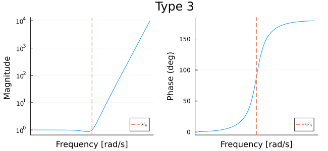
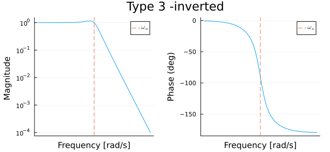
[(ωnjω)2+2ζωnjω+1]±1
For example consider for some constant K the transfer function,
K⋅G(s)=Ks(s2+2s+4)s+3,
where s is the complex frequency variable jω. It can be written as
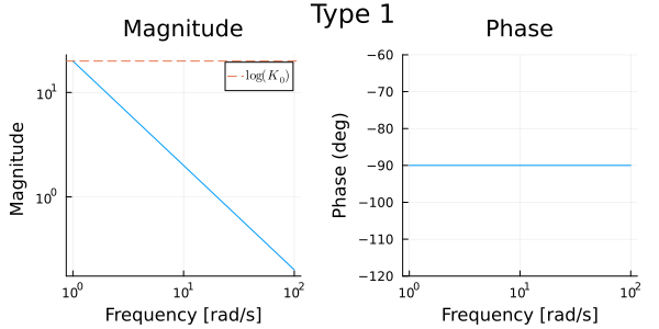
It is a linear function of logω; hence it gives a line of slope n passing through the value log∣K0∣ at ω=1. This line is called a low-frequency asymptote.
In our example above, we had K0(jω)−1. Its magnitude plot is shown in the figure below.
For Type 1 factor, its phase is
∠K0(jω)n=∠(jω)n=n∠jω=n⋅90∘.
The phase is therefore a constant independent of ω.
In our example above, we had K0(jω)−1 . Its phase plot is shown above. In this example the phase is −90∘ for all ω.
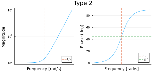
To study ∣jωτ+1∣ and ∠(jωτ+1) as a function of ω, we will look at different cases as below:
For ωτ≪1, we have jωτ+1≈1.
For ωτ≫1 we have jωτ+1≈jωτ.In the case, Type 2 factor behaves like Type 1 with K0=τ,n=1
This transition from one extreme to the other can be said to occur at ωτ=1⟺ω=1/τ.This frequency is called the breakpoint frequency.
For the magnitude plot,
For small ω below the breakpoint, M≈1, a horizontal line.
For large ω above the breakpoint,
logM≈log∣jωτ∣=logωτ=logτ+logω.
This gives a line of slope 1 passing through the point (1/τ,1) on a plot of log-log scale. Note these are just asymptotes; the actual value of M at ω=1/τ is 2 The figure below shows the magnitude slope "steps up" by 1 at the breakpoint.
As for the phase plot,
For small ω (below breakpoint), ϕ≈0∘.
For large ω (above breakpoint),
ϕ≈∠(jωτ)=90∘.
At breakpoint (ωτ=1),
ϕ=∠(j+1)=45∘.
The figure above shows that the phase "steps up" by 90∘ as we go past the breakpoint.
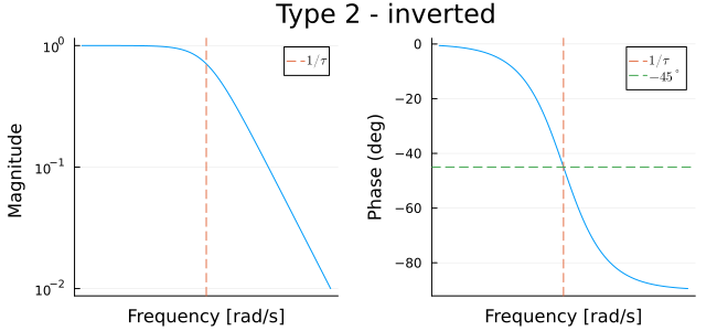
Since this type of factor is the inverse of the one we just discussed, the magnitude and phase plots are reflections of the corresponding plots for the stable real zero with respect to the horizontal axis,
at breakpoint frequency, its magnitude plot “steps down” by 1 in magnitude slope and
Similar to the type 2 case, now the phase and magnitude plots are reflected about the x axis as shown in the plot below.
This brings us to the end of our discussion on creating phase/magnitude plots for the Bode primitives. Next lecture we will do a full fledged example but before that we wrap up the current one with a discussion of resonant frequency.
if we set z:=ωnω as a new variable we can examine the new function M(z). As a function of z, the function M(z) attains a maximum when z=±1−2ζ2.
Answer: Full derivation is left as an exercise. However, one proceeds by differentiating M(z) with respect to z. The derivative is zero at extremal points so we can solve for z from M′(z)=0. Discarding the z=0 solution for obvious reasons we get the above statement
This means ω=ωn1−2ζ2 since ωn cannot be negative. Furthermore we see that there is an extremum for real valued ω only for ζ∈[0,2−1/2]. This ωr:=ωn1−2ζ2 is called the resonant frequency defined above - a frequency at which bad thingscan happen. Here, though, is a more fun video on resonance:
Finally, second order systems are bi-parametric - i.e. while the general shape of the magnitude/phase plots are as discussed above, the exact nature depends on both ωn as well as ζ. This link allows one to change these parameters to visualize how the plots change.