Lecture 05

Reading material: Section 2.2 & 2.4 of the textbook.

Recap

Last time we discussed some common types of signals, the decibel scale, as well as definitions of some common statistics related to signals (mean, variance, SNR, correlation etc.). Today we continue the same topics albeit with a bit more emphasis on implementation details and try to close out Chapter 2.

Correlations & orthogonality

Recall from last time the definition we had for Pearson correlation:

In particular, we showed that if $x$ and $y$ are zero-mean signals then we can write: which in vector notation can be written as:

$$r(x, y) = \sum \limits _{k=1} ^N \frac{x_k y_k}{\sqrt{\sum x_i^2 } \sqrt {\sum y_i^2}} = \dfrac{x^Ty}{\|x\|\|y\|}$$

The quantity in the numerator after the second equality is often written as

$$\langle x, y \rangle := x^T y = \sum \limits _{k=1} ^N x_k y_k$$

and called the inner product between two vectors. We say two vectors are orthogonal if their inner product is zero.

Question: What is the inner product of a vector with itself?

Orthogonality of vectors and signals are important concepts that will show up later. However, for now it suffices to understand why the term orthogonality shows up. Let $u = (a, b)$ be a vector on the plane. The animation below shows this vector $u$ along with the construction: $v=(-b, a)$. Note that $\langle u, v \rangle \equiv 0$!.

This concept extends to higher dimensions as well as to continuous time signals^[1]. Note that the choice of inner product can change depending on the type of "vector" as long as it satisfies some mathematical properties. For example, in the below exercise, we make use of an inner product defined via integration for continuous time signals.

Question: Let $f_n(t) = e^{int}$ be functions for $n \in \mathbb{Z}$ defined via the Euler identity from Lecture 03. Show they are orthogonal under the inner product defined by

$$\langle f, g \rangle := \dfrac{1}{2\pi} \int \limits _0 ^{2\pi} f(t) \overline{g(t)} dt$$

where $\overline{g(t)}$ is the complex conjugate of $g(t)$.

As we will see later, the above result is the cornerstone of the Fourier series and expansion that we will see in later chapters. For now we will leave the reader to work out the following.

Question: Use the above result and Euler's identity to show that $f= \sin(nt)$ and $g = \cos(mt)$ where $m, n \in \mathbb{Z}$ are orthogonal.

The problem with correlation

We will revisit the topic of orthogonality of sines & cosines later; but for now we are faced with a problem. Given an unknown signal $x$, if we compute its correlation with a reference $y$, the value of the correlation can be zero even if the waveforms are identical (consider $x=\sin(x)$ and its time shift: $\sin(x - \pi/2) = \cos(x)$ which is orthogonal to it). Thus, we might get that the correlation between a signal and its own time shift might be zero as illustrated in the below figure!

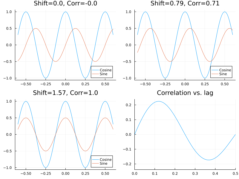
As we can see in the above figure we have a sine wave and a cosine wave of 2 Hz frequency with the panels showing the sine wave shifted by $\pi/4$ and $\pi/2$ units and yielding different levels of correlation with the reference cosine wave.

To get around this limitation, it is common to perform correlations between a signal $x(t)$ and all possible shifts of the reference $y(t)$ and then use the maximal correlation found. The shifts involved are often called lags and the procedure of computing correlation between $x$ and lagged versions of $y$ commonly called cross correlating. Mathematically, for each lag $k$ (or lag variable $\tau$ in continuous time) we have:

$$r_{xy}[k] = \dfrac{1}{N} \sum \limits _{n=1}^N x[n] y[n+k] \qquad \textrm{and} \quad r_{xy}(\tau) = \dfrac{1}{T} \int \limits _0 ^T x(t) y(t+\tau) dt$$

The very last plot above and the equations deserve a little bit of explanation. The bottom right figure shows correlation values (un-normalized) on the y-axis and lags on the x-axis. The last plot is thus generated by computing many correlation values at each possible lag.

Question: Can you work out why the maximum correlation is attained at 0.125 seconds?

Given two signals, as in the figure below, it is not immediately clear how to implement the above formula since shifting the signal leaves it undefined what multiplication should be performed for certain indices. It is commonly accepted to zero pad the signals after shifting so that the correlation is still computed between signals of the same length. Thus, in common implementations, the lag vector ranges from $-N+1$ to $N-1$. The figure below indicates zero padding being performed for a lag of 3 units.

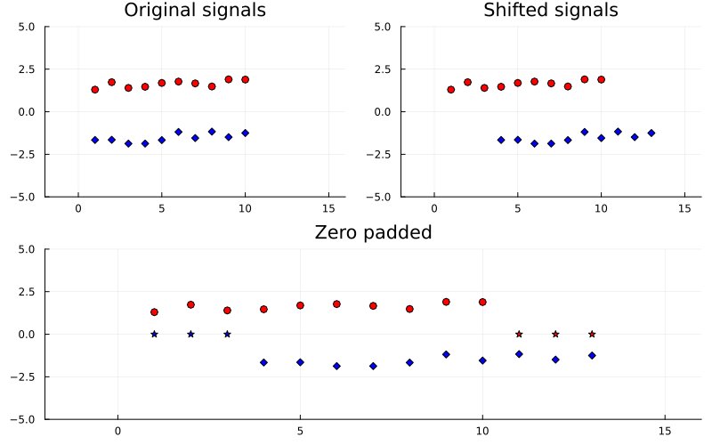
It is because of this implementation detail, i.e. zero-padding that the absolute value of the negative correlation at 0.375 seconds in the previous figure is less than the positive correlation at 0.125 seconds.

Note that while we visualized how to perform cross correlation with zero padding for two equal sized vectors; in reality there is nothing preventing us from adopting the same procedure for finding lagged cross correlations between vectors of differing lengths. The next exercise illustrates this case.

Question: Find the lagged cross-correlation between

and assuming $x$ is a zero-mean vector.
Answer: For simplicity we calculate the un-normalized correlation. Given vectors of length $m$ and $n$, we expect to perform $m+n-1$ lagged correlations. These 7 correlation calculations are shown below along with their corresponding lags:

MATLAB implementation

The following code is taken from CSSB and is an implementation of the lagged cross-correlation function for vectors of the same length with zero-padding.

function [rxy lags] = crosscorr(x,y)
% Function to perform cross correlation similar to MATLABs xcorr
% This version assumes x and y are vectors of the same length
% Assumes maxlags = 2N -1 
% Inputs
%   x       signal for cross correlation
%   y       signal for cross correlation
% Outputs
%   rxy     cross correlation function
%   lags    shifts corresponding to rxy

lx = length(x);			% Get length of one signal (assume both the same length)
maxlags = 2*lx - 1;     	% Compute maxlags from data length
x = [zeros(lx-1,1); x(:); zeros(lx-1,1)]; % Zero pad signal x
for k = 1:maxlags
    x1 = x(k:k+lx-1);         	% Shift signal
    rxy(k) = mean(x1.*y(:));    % Correlation (Eq. 2.30) 
    lags(k) = k - lx;         	% Compute lags (useful for plotting)
end

Exercise: Does the above code assume the inputs are row vectors or column vectors? Modify the above MATLAB function to work for inputs of differing length.

Introduction to filtering

In this section we change gears a bit and discuss filtering; a rich topic in its own right. Recall that we said the definition of signal and noise are relative terms; i.e. what is pertinent to our analysis is our signal and everything else can be termed noise. It is no surprise then that we seek to have techniques to eliminate or reduce noise levels compared to signals in our observation or analysis of systems.

Averaging to reduce noise

One easy way to reduce variability in our observation is to take multiple measurements and then take an average. This ties well with our intuition that as we consider more and more samples/observations/measurements the likelihood of us approaching the true distribution of the data increases.

Consider the following plot which consists of multiple measurements of body temperature taken with a thermometer that is only accurate to $\pm 2^\circ$ F (not a very good thermometer). The true body temperature is marked with a blue line.

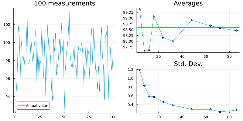
The right side panels show how increasing the number of samples and averaging them let us approach the true value over repeated measurements. Further, it can be shown that the "error" scales as $\sqrt{N}$ when considering the mean of $N$ measurements. This observation can be verified in the above plot.

Question: CSSB states that

When multiple measurements are made, multiple values or signals are obtained. If these measurements are combined or added together, the means add so that the combined value or signal has a mean that is the average of the individual means.

Suppose we have $m$ sets of measurements, $S_1, S_2, \dots S_m$ where each set $S_k$ has size $N_k$ and mean $\mu _k$. Call the entire collection of measurements as $S = \{S_1, S_2, \dots, S_m\}$. Is it true that the average of the means $\mu_k$ is the same as the mean $\mu _S$ of $S$?

Ensemble averaging

CSSB (and therefore our course) refers to constructing a single timeseries/signal out of multiple ones by averaging them in time (technically pointwise) as ensemble averaging.

The idea here is the same: averaging reduces variability and thus might enable one to see systemic patterns not obvious by examining individual signals. Consider for example the very noisy sinusoid from Lecture 03 reproduced here in the left plot. Taking 50 such noisy sinusoids and averaging them pointwise reduces the noise artifact.

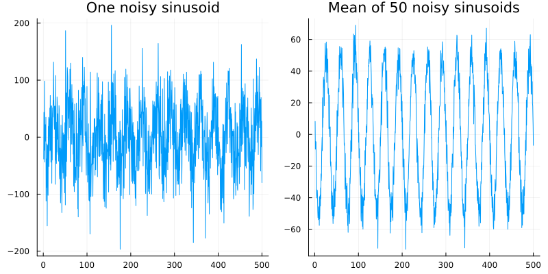
Section 2.4.4 of CSSB for further details.

[back]

[1]	Actually it applies to all vector spaces that can be equipped with an inner product but we will not get to that level of abstraction in this course.