3.
Cooling
Schedule
As mentioned in the introduction, the choice of the cooling schedule is crucial to the convergence of the algorithm to a global minimum. By cooling schedule[15], we mean the choice of the following parameters:
1. Initial temperature
2. Final temperature
3. Length of Markov Chains
4. A rule for changing the current value of the control parameter, i.e Tn+1 as function of Tn
3.1
Initial Temperature
Choosing a very high initial temperature results in a lot of
time being wasted at the beginning stage of the search. However, a very low initial temperature
could result in the system being trapped in a local potential energy minimum,
because the configuration space was not sufficiently explored. We found that
the optimal choice of initial temperature depends on the cluster size: the
larger the cluster, the higher the initial temperature. In this project, the
initial temperature is chosen so that the initial acceptance ratio is around
80%.
3.2
Final Temperature
In theory, the annealing process should terminate at zero Kelvin. This, however, is not feasible from a practical standpoint since, in all likelihood, the system would have converged to its final configuration before attaining zero. There is also a question of singularity when implementing the Metropolis criterion at close to zero temperature. A more practical approach, adopted in this project, is to terminate the program based on a predetermined minimum acceptance ratio.
3.3
Decrement Rules for the Temperature
As mentioned in the introduction, one of our primary objectives is to incorporate information obtained on the structural evolution of the system into the cooling schedule. This is done via the temperature decrement rate. Figure 1 below shows a plot of “specific heat”, calculated from the variance of the potential energy, for a cluster of four atoms using a fixed decrement rate of 0.99, i.e.
![]() (3.1)
(3.1)
It can be seen that
the curve is essentially flat for close to five orders of magnitude in temperature.
A rapid change in the curve occurs at temperature, ![]() . From statistical mechanics we know that divergence in
specific heat is an indication of onset of a phase transition, in our case the
inception of cluster formation. From this example, it is obvious that a
decrement rate that is fast in the “flat regions” but slows down at the onset
of cluster formation, indicated by rapid change in Cv, would result a more
effective algorithm than the fixed rate method. Such was the motivation behind
our proposed decrement rule.
. From statistical mechanics we know that divergence in
specific heat is an indication of onset of a phase transition, in our case the
inception of cluster formation. From this example, it is obvious that a
decrement rate that is fast in the “flat regions” but slows down at the onset
of cluster formation, indicated by rapid change in Cv, would result a more
effective algorithm than the fixed rate method. Such was the motivation behind
our proposed decrement rule.
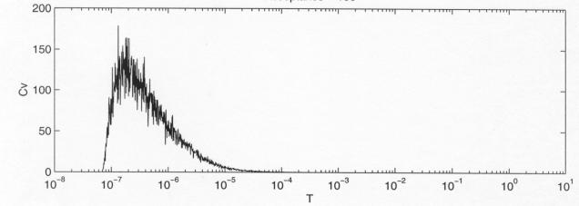
Figure 1. Plot
of specific heat as a function of temperature for a fixed temperature decrement
rate of 0.99.
While there are many candidates for the functional dependence of decrement rate with Cv, we proposed the following two rates. The first, a modified form of a decrement rate initially proposed by Aarts and Laarhoven[16], is given as
![]() “Inverse” (3.2)
“Inverse” (3.2)
The second originally suggested by Huang et al.[17] is
![]() “Exponential” (3.3)
“Exponential” (3.3)
where the adjustable parameter, ![]() , is positive definite and smaller than unity. Discussion on
how to go about selecting
, is positive definite and smaller than unity. Discussion on
how to go about selecting ![]() is given in the
results section.
is given in the
results section.
The specific heat, Cv, is calculated from the fluctuation of the potential energy at each temperature:
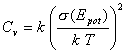 (3.4)
(3.4)
3.4
Markov Chain
The Simulated Annealing is best described, mathematically, by a Markov process. A Markov process is a sequence of trials, where the outcome of each trial depends on only on the outcome of a previous one. In the case of simulated annealing, trials correspond to transitions between an initial configuration at a fixed temperature to another all the way to the global minimum. Each Markov chain in simulated annealing is generated at fixed temperature. The mathematical theory of simulated annealing is beyond the focus of this project. Only a summary of the essential results will be discussed here. A detailed treatment is given in an excellent text by van Laarhoven and Aarts[15] . According to the theory, asymptotic convergence of the simulated annealing algorithm is guaranteed if the Markov chain is irreducible and of infinite length. A Markov chain is irreducible, if and only if for all pairs of configurations (i, j) there is a positive probability of reaching j from i in a finite number of transitions. As a result of the irreducibility condition, the transition matrix, P, must satisfy the following conditions:
(3.6)
![]()
![]()
The largest eigenvalue of P must also be equal unity. A sufficient, but not necessary condition for irreducibility of the Markov chain is detailed balance. The Markov chain length is determined by stipulating the minimum number of configuration to be accepted at every temperature level so as to minimize the noise in the Cv data used in the computation of the decrement rate. This is further discussed in the next section.