5.
Results
and Discussion
5.1 Optimization conformation for different Silicon
clusters
Global optimal conformations for silicon clusters
up to 14 atoms have been found using the code developed. Table 1 shows the
minimum potential energies per atom found for different clusters. These minimum
energies agree with published data in the literature[9].
Table 1. Minimal Energy obtained for different size silicon
clusters
|
Cluster size |
Energy per atom |
Cluster size |
Energy per atom |
|
3 atoms |
-0.8085 |
9 atoms |
-1.5649 |
|
4 atoms |
-1.0004 |
10 atoms |
-1.5800 |
|
5 atoms |
-1.2783 |
11 atoms |
-1.6661 |
|
6 atoms |
-1.3749 |
12 atoms |
-1.6245 |
|
7 atoms |
-1.4418 |
13 atoms |
-1.6494 |
|
8 atoms |
-1.5111 |
14 atoms |
-1.6464 |
Note: Energies are in reduced unit as explained in the potential
section.
Figure
3 shows the initial and optimal configuration for clusters ranging from 4 to 13
atoms.
4 atoms 5
atoms


6 atoms 7
atoms


8 atoms 9
atoms


10 atoms 11
atoms


12 atoms 13
atoms
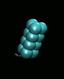

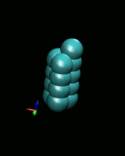

Figure 3. Initial and
optimal configuration of n-atom Silicon
clusters (n = 4-13). Clusters were visualized with VMD[10].
5.2
Cluster evolution
to stable orientation
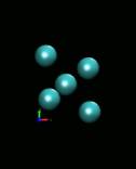
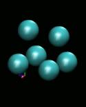
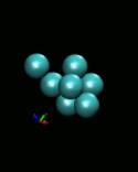
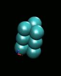
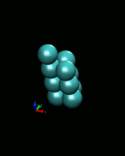
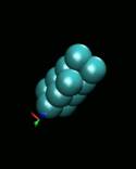
Figure 4 illustrates the structural and energy evolution of
an eight atom cluster during implementation of a simulated annealing process.
The atoms are colored differently for purpose of illustration. Each color represents one specific atom as it
is perturbed throughout the annealing process.
Arrows indicate the direction of temperature decrease.
![]()


![]()
![]()
Figure 4. Typical structural evolution of 8 atom
cluster. Energy is in reduced units of
ε = 2.17eV. Final frame represents
potential energy global minimum.
5.3
Costs of each
algorithm
Table 2 shows the function cost for the decrement rules
tested. The comparison was conducted for 5 different cluster sizes. Each value represents an average of at least
five trials performed. It can be seen
from the table that the proposed decrement rates performed better than the
fixed decrement rule with the exponential rule showing the best performance.
Table 2. Comparison of
temperature decrement performance.
|
|
Exponential |
|
Fixed |
|
Inverse |
|
|
natoms |
function cost |
error |
function cost |
error |
function cost |
error |
|
4 |
65646 |
30371 |
326400 |
32883 |
78900 |
9200 |
|
6 |
72148 |
33860 |
323124 |
41990 |
204490 |
9535 |
|
8 |
129792 |
50629 |
461095 |
14935 |
365271 |
47136 |
|
10 |
139974 |
45833 |
591374 |
17846 |
481550 |
113470 |
|
12 |
249351 |
71782 |
690491 |
21244 |
589149 |
93077 |
The CPU time for the inverse scheme is shown in Figure
5. These results were obtained on an
IBMF-80 server, 450 MHz RS64C and utilized a gcc compiler, utilizing a delta
value of 0.001. Each value represents
an average of at least five trials performed. The computational time in this
example scales as approximately N3 . This should not be understood
as the scaling power of the algorithm! To obtain the scale, more atom cases
need to be considered. Unfortunately, we were unable to achieve this due to
time limitations.
Figure 5. CPU time for
inverse temperature decrement scheme.
5.4
One atom versus
multiple atom perturbation
For various cluster sizes and both temperature decrement
schemes one atom perturbation versus multiple atom perturbations were examined.
It was found that the multiple
perturbations were on average 7-15% more efficient in reaching convergence in
terms of the number of function calls.
5.5
Comparison with GA
Genetic algorithms (GAs) have also been utilized to solve
global optimization problems[11,12]. The GA as it is known today was developed by
John Holland in the 1960’s[13,14].
The GA uses principles based on Darwinian natural evolution
theories. “As many more individuals of
each species are born than can possibly survive, and as consequently there is a
frequently recurring struggle for existence, it follows that any being, if it
vary in any manner profitable to itself, under the complex and sometimes
varying conditions of life, will have a better chance of survival and thus be
naturally selected. From the strong principle of inheritance, any selected
variety will tend to propagate its new and modified form” (The Origin of
Species, Darwin, 1859). These
principles are incorporated in the genetic algorithm framework. Specifically,
the survival of the fittest and evolution are used when selecting candidate
solutions (in this case the coordinates of the cluster structure represents one
possible solution) in the total population (all available cluster structures
and their corresponding coordinates).
These candidate solutions compete with each other for survival. Through breeding, selection, and mutation
operations the fittest individuals pass their genetics on to subsequent
generations. Following several
generations the individual that is fittest in the population should be the
fittest possible (global potential energy minimum attained).
Iwamatsu[9]
employed a GA for Si cluster optimization for 3-11 atoms with both the
Stillinger-Weber and Gong potentials. As mentioned earlier, our minimum energy
configurations are in good agreement with theirs. Figure 6 below compares the function cost of the GA algorithm, as
presented in Sastry and Xiao’s project report, with those obtained using the
exponential decrement rule. Although it appears from the plot that the newly
implemented schedule is more efficient for cluster sizes ranging from 6-12
atoms, we think such a conclusion can not be made because of the small size of
the systems considered. Furthermore, it can be argued that the results
displayed are not the optimal for both algorithms.
Figure 6. Algorithm costs for the exponential
scheme and the Sastry and Xiao[6] genetic algorithm.
5.5 Choice
of delta for each algorithm
The selection of the delta parameter in the inverse and
exponential cooling schemes is critical to the solution converging to a local
minimum as discussed above. Figure 7 shows
delta sensitivity for both cooling schemes and how it relates to the function
cost. The inverse formula exhibits a
region of robustness for convergence to the global minimum between 0.0005 and
0.006. Outside of this region, this
algorithm does not converge to the global minimum. The exponential cooling scheme demonstrates convergence at a
delta ranging from 0.0001 to 0.0015.
Figure 7. Delta sensitivity of temperature decrement
rules. The x’s indicate deltas where
the global minimum was not obtained.
The solid diamonds represent solutions which converged to global optimum
structure.
5.6 Choice
of number of inner loops (k*natoms) for each algorithm -
Figure 8 demonstrates the sensitivity of the inner loop
(k*natoms) for the inverse, exponential, and fixed temperature decrement
schemes. All three schemes will not
converge when too small of an inner loop size is chosen (for example 50). However, if too large of an inner loop size
is chosen, computer time is wasted.
Therefore, we were careful to select this parameter to strike a balance
between these factors. We generally
implemented a factor of 50*natoms, since the inner loop length also depends on
the number of atoms within the cluster.
Figure 8. Inner loop sensitivity of various
temperature decrement schemes. The x’s
indicate deltas where the global minimum was not obtained. The solid diamonds represent solutions which
converged to global optimum structure.