Accessing diffusion data and computing diffusivity

We will work with the traditional “five frequency” model for solute diffusion in a face-centered cubic (FCC) lattice. A relatively large database of solute barriers was published by the Dane Morgan group recently; paper with the public database which we will use for our computation.

import pandas as pd
import numpy as np
from numpy.random import default_rng
rng = default_rng()
import seaborn as sns
import matplotlib.pyplot as plt
import scipy.constants
# grab Boltzmann's constant; we'll need it later
kBoltzmann = scipy.constants.physical_constants['Boltzmann constant in eV/K'][0]

The datafile we need is an Excel spreadsheet, available at https://ndownloader.figshare.com/files/12753815. In addition, you should investigate the structure of the database at https://figshare.com/articles/dataset/DFT_dilute_solute_diffusion_in_Al_Cu_Ni_Pd_Pt_and_Mg/1546772

We use sheet_name=None to get all of the sheets; the first sheet is the host information, followed by different solutes.

Some information about what we’re going to see:

• The first sheet is “host information”; it has the element name, crystal structure, lattice constant, vacancy formation energy. In addition, the Morgan group identifies a “correction shift” A_shift and energy shift E_shift that they apply to the diffusivity data, of the form \(A_\text{shift}\exp(-E_\text{shift}/k_\text{B}T)\).
• Each subsequent sheet has all of the solute data, which includes the hop barriers and attempt frequencies

diffusionDB = pd.read_excel('https://ndownloader.figshare.com/files/12753815', 
                            sheet_name=None)

You’ll want to inspect the content of the sheets to understand what the data looks like.

diffusionDB.keys()

dict_keys(['Host Information', 'Al-X', 'Cu-X', 'Ni-X', 'Pd-X', 'Pt-X', 'Mg-X', 'W-X', 'Mo-X', 'Fe-X', 'Au-X', 'Ca-X', 'Ir-X', 'Pb-X', 'Ag-X', 'Zr-X'])

diffusionDB['Host Information']

Let’s work with Aluminum, and examine the information available for the host:

host_element = 'Al'
diffusionDB['Host Information'][host_element]

0          FCC
1          933
2       0.4847
3     4.039094
4          NaN
5           12
6          0.2
7          NaN
8          NaN
9          NaN
10         NaN
11         NaN
Name: Al, dtype: object

We’ll need to grab some of this information for later:

a0 = diffusionDB['Host Information'][host_element][3]
Evform = diffusionDB['Host Information'][host_element][2]
A_shift, E_shift = diffusionDB['Host Information'][host_element][5], diffusionDB['Host Information'][host_element][6]

We can investigate the solute data sheet:

solute_elements = host_element + '-X'

And we select one species (Ag) to consider:

soluteZ = 47
diffusionDB[solute_elements][soluteZ]

0           Ag
1      0.58143
2      0.57299
3      0.45938
4      0.59649
5      0.52671
6     4.224243
7     4.202993
8     1.322896
9     4.226324
10     4.17018
11    0.040325
12    1.141065
13         NaN
14         NaN
15         NaN
16         NaN
Name: 47, dtype: object

Let’s grab data for that particular solute:

df = diffusionDB[solute_elements][soluteZ]
solute = df[0]
barriers = df[1:6].astype('float').to_numpy()
attempt_freq = df[6:11].astype('float').to_numpy()
D0_diff, Q_diff = df[11], db[12]
print(barriers)
print(attempt_freq)
print(solute, D0_diff, Q_diff)

[0.58143 0.57299 0.45938 0.59649 0.52671]
[4.22424298 4.20299328 1.32289592 4.22632423 4.17017994]
Ag 0.0403254943845161 1.14106512869029

To compute solute diffusivity, we need to know how to transform this data into diffusivity. There are a few steps involved:

1. Converting hop activation barriers and attempt frequencies into rates: the titular “five frequencies” of the model.
2. Converting the rates into diffusivity.

The former is done using the Arrhenius relation; for activation barrier \(Q\) and attempt frequency \(\nu\) at temperature \(T\), the rate \(w\) is \[w = \nu \exp\left(-\frac{Q}{k_\text{B} T}\right)\] where \(k_\text{B}\) is Boltzmann’s constant.

The latter is done using the closed-form expression for the five-frequency model. The rates are

• w0: vacancy hop rate; independent of the solute, only dependent on the host.
• w1: vacancy swing rate: jump rate for a vacancy next to a solute, jumping to another neighbor site of the solute
• w2: solute exchange rate: jump rate for a solute to jump into the vacant site
• w3: vacancy escape rate: jump rate for a vacancy next to a solute, jumping away from the solute
• w4: vacancy capture rate: jump rate for a vacancy away from a solute, jumping next to a solute

Note that the ratio \(p=w_4/w_3\) is the enhancement probability for a vacancy to be found next to a solute; \(p>1\) means that vacancies are attracted to the solute, and \(p<1\) means that vacancies are repelled by solutes. The derivation of the five frequency diffusivity is a bit complex. Note that when \(w_2\) is very small, the diffusivity is proportional to \(p\cdot w_2\), but when \(w_2\) is very larger, the diffusivity is proportional to \(p(w_1 + w_3 F/2)\) where \(F\) is a correlation factor. The expression for the diffusivity is: \[D = a_0^2 c_\text{v} f(w_0, w_1, w_2, w_3, w_4)\] for lattice constant \(a_0\), equilibrium vacancy concentration \(c_\text{v} = \exp(-E^\text{form}_\text{v}/k_\text{B}T)\) and five-frequency function \(f\).

def fivefreq(w0, w1, w2, w3, w4):
    """The solute diffusion correlation factor in the 5-freq. model"""
    b = w4 / w0
    F7 = 7. - b * (1338.1 + b * (924.3 + b * (180.3 + b * 10.))) / \
              (435.3 + b * (596. + b * (253.3 + b * (40.1 + b * 2.))))
    p = w4 / w3
    return p * w2 * (2. * w1 + w3 * F7) / (2. * w2 + 2. * w1 + w3 * F7)

def Arrhenius(Q, nu, T):
    """Takes activation barrier Q in eV, nu in THz, T in K, and returns a rate in THz"""
    return nu*np.exp(-Q/(kBoltzmann*T))

Arrhenius(1.0, 1.0e12, 300)

1.5875937551666036e-05

Now, try comparing the Arrhenius fit for the solute data against the direct five-frequency calculation:

T = 600
D = Arrhenius(Q_diff, D0_diff, T)
D

1.049674050545576e-11

cV = Arrhenius(Evform, 1., T)
w = Arrhenius(barriers, 1e12*attempt_freq, T)
(a0*1e-8)**2 * cV * fivefreq(*w) * Arrhenius(E_shift, A_shift, T)

1.0718133901395067e-11

Uncertainty quantification

We can apply an approach similar to that used in Uncertainty quantification of solute transport coefficients: with an empirical estimate of the covariance matrix, we can generate sample activation barriers, and determine the distribution of predictions of diffusivity.

Our empirical correlation matrix for this model is below. It is approximate, with a form similar to that found for solutes in HCP Mg. In this case, it is a \(6\times 6\) matrix, with the first entry for the vacancy formation energy, followed by the 5 rates. There is an anticorrelation between the rates w3 and w4, along with reduced correlation with the vacancy formation energy.

barrier_covariance = 0.003*np.eye(6) + 0.003*np.ones((6,6))
barrier_covariance[4,5] = -0.001
barrier_covariance[5,4] = -0.001
barrier_covariance[0,5] = 0.
barrier_covariance[5,0] = 0.
barrier_covariance

array([[ 0.006,  0.003,  0.003,  0.003,  0.003,  0.   ],
       [ 0.003,  0.006,  0.003,  0.003,  0.003,  0.003],
       [ 0.003,  0.003,  0.006,  0.003,  0.003,  0.003],
       [ 0.003,  0.003,  0.003,  0.006,  0.003,  0.003],
       [ 0.003,  0.003,  0.003,  0.003,  0.006, -0.001],
       [ 0.   ,  0.003,  0.003,  0.003, -0.001,  0.006]])

np.linalg.eigh(barrier_covariance)

(array([8.00831974e-05, 3.00000000e-03, 3.00000000e-03, 3.00000000e-03,
        7.86296696e-03, 1.90569498e-02]),
 array([[-2.73008069e-01, -7.51468311e-01, -1.59955093e-01,
          2.03196193e-01,  3.66220423e-01, -3.99712708e-01],
        [ 3.38527167e-01,  2.80877441e-01, -1.31172585e-02,
          7.69407845e-01, -9.78281429e-02, -4.52522243e-01],
        [ 3.38527167e-01,  8.47034804e-02, -6.65704257e-01,
         -4.69803996e-01, -9.78281429e-02, -4.52522243e-01],
        [ 3.38527167e-01, -1.77713844e-01,  7.18810288e-01,
         -3.50402898e-01, -9.78281429e-02, -4.52522243e-01],
        [-4.76853148e-01,  5.63601233e-01,  1.19966319e-01,
         -1.52397145e-01,  5.20903278e-01, -3.82109529e-01],
        [-5.95210670e-01, -2.77555756e-17,  1.11022302e-16,
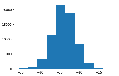
         -1.11022302e-16, -7.52217615e-01, -2.82653353e-01]]))

To generate our random samples, we use the multivariate_normal function. Here is how we can use it to construct a distribution of diffusivities (here, stored as the log of the diffusivities) by generating samples. Note: we need to prepend the vacancy formation energy to the barrier list so that the energies that come out are a vector [Evform, w0barrier, w1barrier, w2barrier, w3barrier, w4barrier].

logD = []
T = 600
Nsamples = 2**16
for ene in rng.multivariate_normal(mean=np.insert(barriers, 0, Evform), 
                                   cov=barrier_covariance, 
                                   size=Nsamples):
    cV = Arrhenius(ene[0], 1., T)
    w = Arrhenius(ene[1:], 1e12*attempt_freq, T)
    D = (a0*1e-8)**2 * cV * fivefreq(*w)
    logD.append(np.log(D))
logD = np.array(logD)

np.mean(logD), np.std(logD)

(-23.936257895471147, 2.7688013872446393)

plt.hist(logD);

To-do:

With this in mind, we want to investigate some questions:

1. Examine the histograms of log diffusivity at different temperatures; is the distribution normal?
2. Does the nonlinearity of the model introduce bias? That is, is the average log diffusivity the same as the log diffusivity of the average parameters?
3. Plot the standard deviation of the log diffusivity vs. inverse temperature over a range of physically relevant temperatures. What do you observe?
4. Time permitting, automate the analysis over the whole solute list, and identify any outliers.