In this example, we shall use OOF2 to use the finite
element method to analyze the physical behavior of a bimetallic strip.
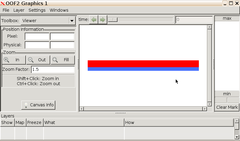
The strip is comprised of two sheets of metal bonded together at an
interface, as indicated below. The properties and geometry of the strip
in the dimension coming out of the plane of the paper are assumed to be
quasi-infinite uniform, allowing a two-dimensional treatment of this
system. In this system, the upper (red) layer is copper, bonded to a
lower (blue) layer of carbon steel.
The differential thermal expansion of the two metals upon heating or cooling causes structural deformation of the strip, and is exploited in thermostatic feedback loops in domestic ovens and other appliances to maintain fixed chamber temperatures.
We shall analyze the physical and mechanical behavior of the strip upon heating. Of particular interest is the interfacial stress, which—if it becomes too large—can lead to delamination of the two metals, causing the bimetallic strip to fail and compromising the thermostatic feedback loop.
This guide is neither exhaustive nor comprehensive. To see the full
range of OOF2 features, and explore the details of the
features exhibited within this guide, please see the OOF2
Manual. Hovering your cursor over the options in the OOF2 GUI will
also provide on-demand information about the various options.
Alternatively, you can run any of the interactive tutorials. The
necessary example input files are installed in
/class/mse404ela/OOF2/examples (which is an automount
directory; you will need to access the directory first in order to read
the files).
We will access OOF2 using the local EWS installation;
please load
module load OOF2to proceed. Alternatively, you can use OOF2 via the web
implementation at nanoHUB.org. This
requires an active nanoHUB account (free), and note that you must use
the “Upload/Download” dialog to upload an image file.
N.B. As we have seen, OOF2 has no predefined units, and
we may use any consistent units of our choosing. Throughout this guide
we will employ the SI convention (m, kg, Pa, J, N, etc.).
References
Prepare files, load module. First, load
OOF2 with module load OOF2. Next create your
own local directory for your work, including today’s walkthrough. From
/class/mse404ela/OOF2/Walkthrough, copy the file
bimetallic.png into your local directory.
Start OOF2. After changing into your local
directory, run oof2.
It is instructive to spend a moment reading the text in the
OOF2 welcome pane describing the basic OOF2
workflow. N.B. You can save your work as a Python log
using File | Save. It is strongly recommended that you save
frequently to a Python log file to checkpoint your work.
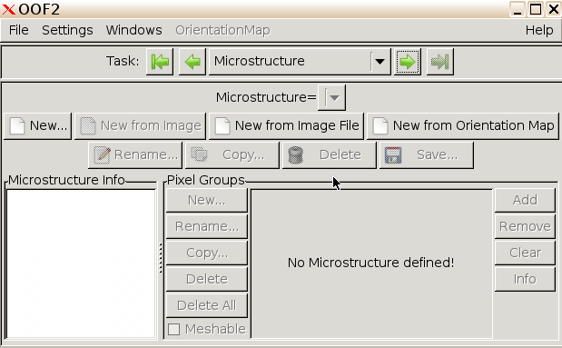
Create microstructure. Change to the
Microstructure task in the main OOF2 window.
Click “New from Image File” in the resulting window.
Select bimetallic.png and set the height to 0.01 m.
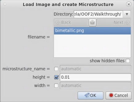
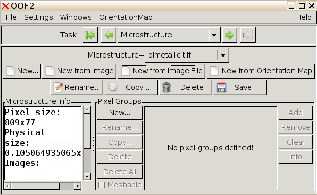
Click OK, and the microstructure window will now contain your uploaded image data.
From the dropdown Windows menu, select
Graphics and click New to see your uploaded
image.
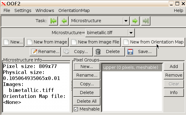
Build Pixel Groups. We shall now inform
OOF2 that we have two separate materials, by forming “Pixel
Groups”.
From the Toolbox menu, select
Pixel Selection, and in the Method menu select
Color.
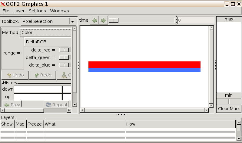
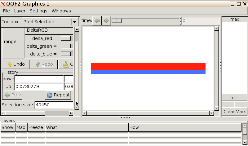
Click on the upper red layer. A value will appear in the Selection Size variable box defining the size of the selected layer.
Drag the “Graphics 1” window out of the way and return to the main
OOF2 window. Click on New... under
Pixel Groups and name the selected group “upper”. Click
OK.
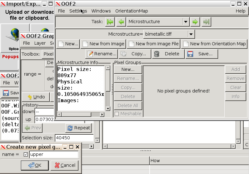
You will see that we have established a new Pixel Group.
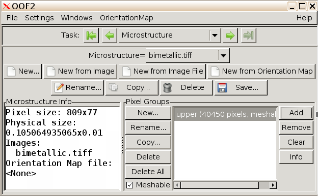
Click the Add button to the right of the window to add
our selected pixels to this group.
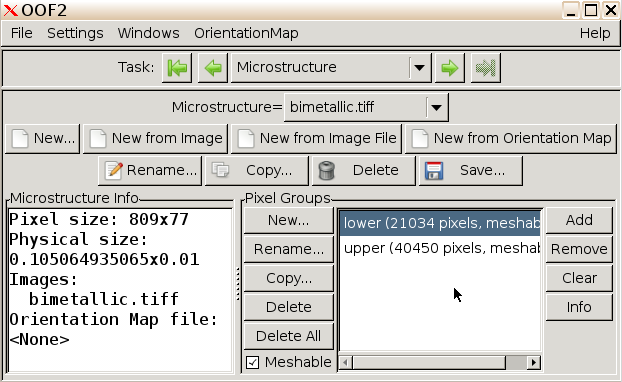
Repeat this process for the bottom layer, to generate a pixel group named “lower”.
Build material properties. We shall now input
the physical properties for each layer in the strip—copper (upper), and
carbon steel (lower). In the main OOF2 window, use the
Task dropdown to navigate to the Materials
pane.
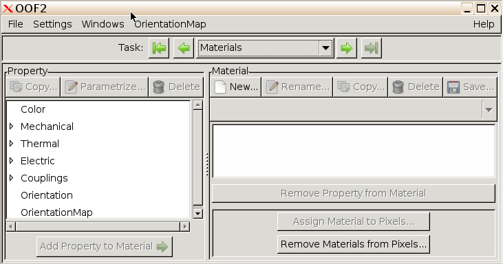
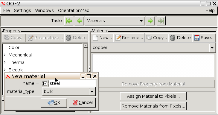
Click New... to add a new material. Name the materials
“copper” and “steel”, and leave their specification as bulk.
We shall now assign the following properties to the two materials:
| Property | Copper | Steel |
|---|---|---|
| Young’s modulus \(E\) [GPa] | 117 | 200 |
| Poisson’s ratio \(\nu\) | 0.33 | 0.27 |
| Thermal conductivity \(k\) [W/m\(^\circ\)C] | 390 | 41 |
| Thermal expansion coefficient \(\alpha_T\) at \(T_0=0^\circ\text{C}\) [K\(^{-1}\)] | \(51\times10^{-6}\) | \(36\times10^{-6}\) |
| Color [R,G,B] | [1,0,0] | [0,0,1] |
Let’s first consider copper.
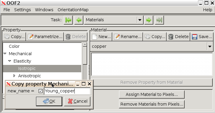
To specify the Young’s modulus, in the Property window
on the left click the triangle to the left of Mechanical,
followed by the triangle to the left of Elasticity, then
highlight the word Isotropic. At the top of the
Property window, click Copy..., name the
property “Young_copper” and click OK.
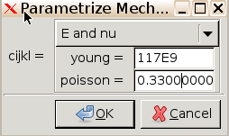
Select Young_copper and click
Parametrize... and in the drop down menu, select
E and nu. Input the values for Young’s modulus and
Poisson’s ratio (\(\nu\)) from the
table above and click OK.
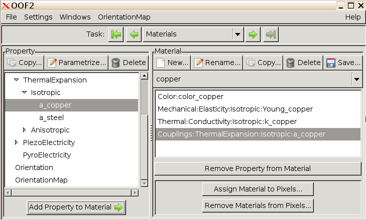
Follow a similar procedure to add the other three properties in the table, accessing the pertinent properties as follows:
| Property | Selection |
|---|---|
| Thermal conductivity, \(k\) | Thermal -> Conductivity -> Isotropic |
| Thermal expansion coefficient, \(\alpha_T\) at \(T_0=0^\circ\text{C}\) | Couplings -> Thermal Expansion -> Isotropic |
| Color | Color |
Attach materials properties. Select copper in
the Material column on the right hand side of the main
OOF2 window. Select each of the four materials properties
we assigned in turn (Young + Poisson, k, alpha, color) in the
Property column on the left side and click
Add Property to Material.
Repeat for steel.
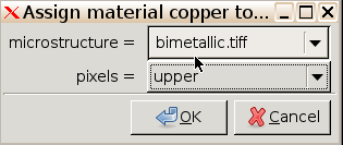
Assign materials to pixel groups. Select copper
in the Material column and click
Assign Material to Pixels.... Choose upper to make the
upper layer of the bimetallic strip copper.
Follow an analogous process to make the lower layer steel.
Generate skeleton. In OOF2, we
first create a “skeleton” of finite elements that we subsequently use to
create the mesh. The skeleton is purely geometric, whereas the mesh
contains element properties and basis functions.
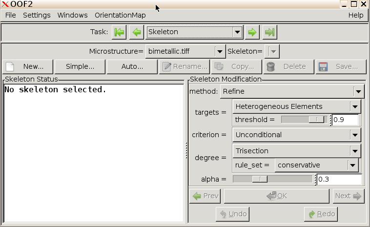
In the main OOF2 window, use the Task
dropdown to navigate to the Skeleton pane.
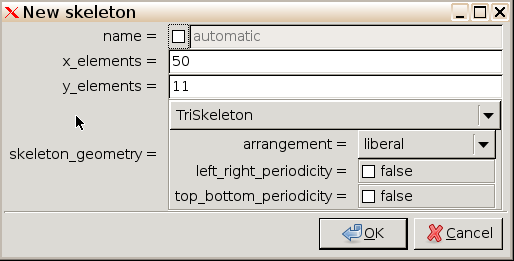
Click New... to specify a new skeleton, and set the
number of x elements to 50, the number of y elements to 11, the mesh
type to TriSkeleton, and the arrangement to Liberal. Click OK.
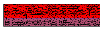
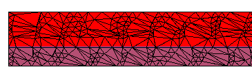
The Graphics window will now display your initial skeleton over your microstructure.
Careful inspection of the skeleton reveals that there are some “heterogeneous elements” containing both copper and steel within their area, and there are too few elements near the interface where we expect large variation in properties.
We shall perform a number of rounds of skeleton refinement to
generate more reasonable domain decomposition using the
Skeleton Modification tools in the right hand column of the
main OOF2 window.
These tools attempt to minimize the skeleton energy, where the energy is defined as a linear combination of a homogeneity and a shape term:
\[E = \alpha E_\text{homogeneous} + (1-\alpha) E_\text{shape}\]
Heterogeneous elements and those with high aspect ratios have high energies. The parameter \(\alpha\) (not to be confused with thermal expansion!) controls the trade-off between these contributions.
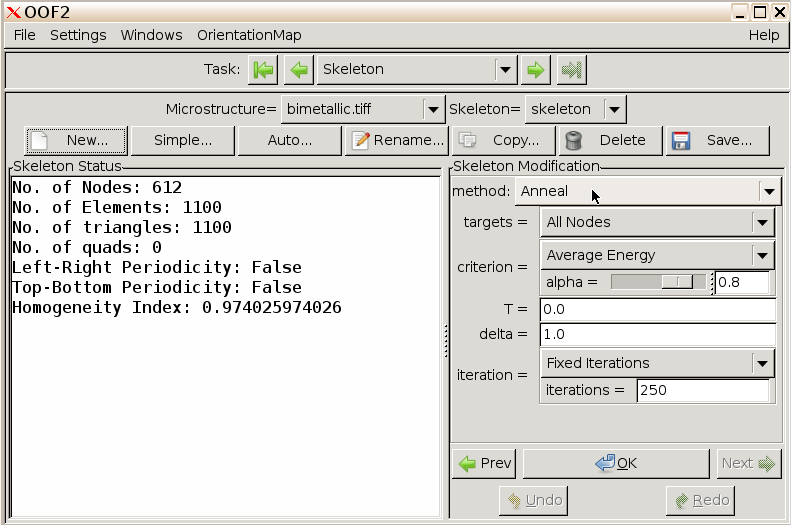
Anneal. This process
attempts to make the elements more homogenous using a random skeleton
refinement protocol similar to simulated annealing. Use as a criterion
“Average Energy” with alpha = 0.9 and specify 100 iterations. T is the
effective temperature, with T=0 permitting only downhill moves in
energy.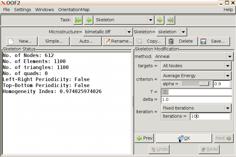
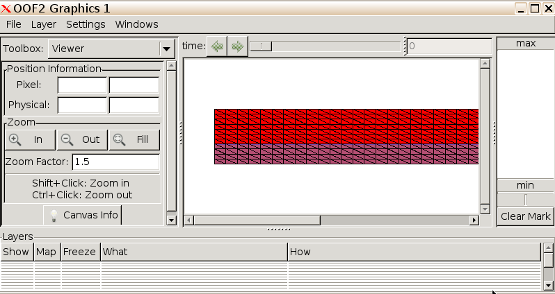
Click OK to perform the annealing procedure. You can watch the skeleton evolve in the Graphics window, and the numerical convergence in the Messages and Activity window.
In the Graphics window, we can access Zoom options via the dropdown Settings menu. Zooming in on the skeleton shows that we have improved alignment of the mesh with the phase boundaries.
Swap Edges to perform a
random flipping of element edges in an effort to achieve better phase
boundary alignment. Use alpha = 0.8. Click OK.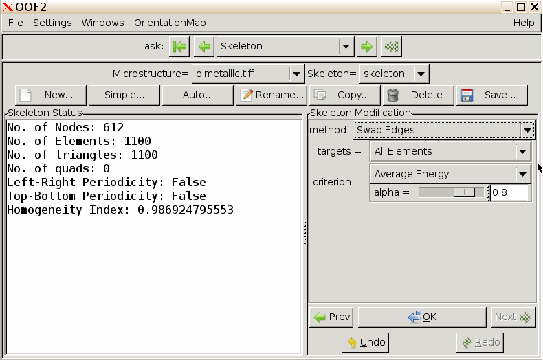

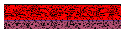
The skeleton is well aligned with the phase boundary, and the homogeneity index is 0.99 indicating excellent alignment with phase boundaries.
(N.B. We will not do this here to save computational time, but we can use the “Refine” method to increase the number of elements. Set the targets to “All Elements”, criterion to “Unconditional”, degree to “Bisection”, rule set to “Liberal” and alpha to 0.8. Click OK.){ width=50% }
Generate mesh. In the main OOF2
window, use the Task dropdown to navigate to the FE Mesh
pane.
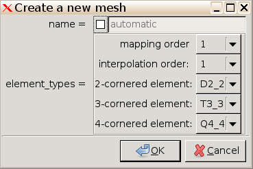
Click New... to generate a mesh based on our skeleton.
Leave mapping order and interpolation order as 1. (For higher
accuracy—at the expense of longer computation times—we may wish to
select 2.) Click OK.
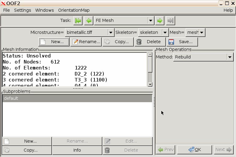
We now have a mesh with properties listed in the left column of the FE Mesh window.
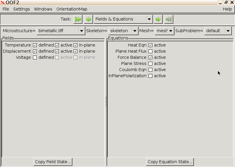
Specify equations. In the main OOF2
window, use the Task dropdown to navigate to the
Fields and Equations pane.
In the Fields column on the left, tick all three boxes
(defined, active, in-plane) in
the rows for Temperature and Displacement.
In the Equations column on the right, tick the boxes
next to Heat Eqn and Force Balance.
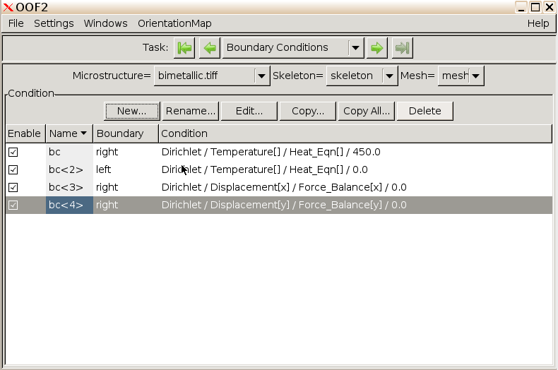
Specify boundary conditions. In the main
OOF2 window, use the Task dropdown to navigate to the
Boundary Conditions pane.
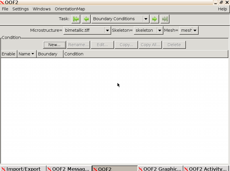
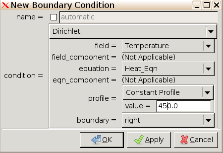
Click New.... Using Dirichlet boundary conditions for
the temperature field, specify the right boundary to \(450^\circ\text{C}\).
Following the same protocol, specify the left boundary to be \(0^\circ\text{C}\).
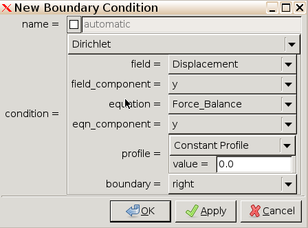
Following a similar protocol, fix the right boundary \(y\)-displacement to zero.
Following a similar protocol, fix the right boundary x-displacement to zero.
We can see the specified BCs in the main OOF2
window.
Solving. In the main OOF2 window,
use the Task dropdown to navigate to the Solver pane.
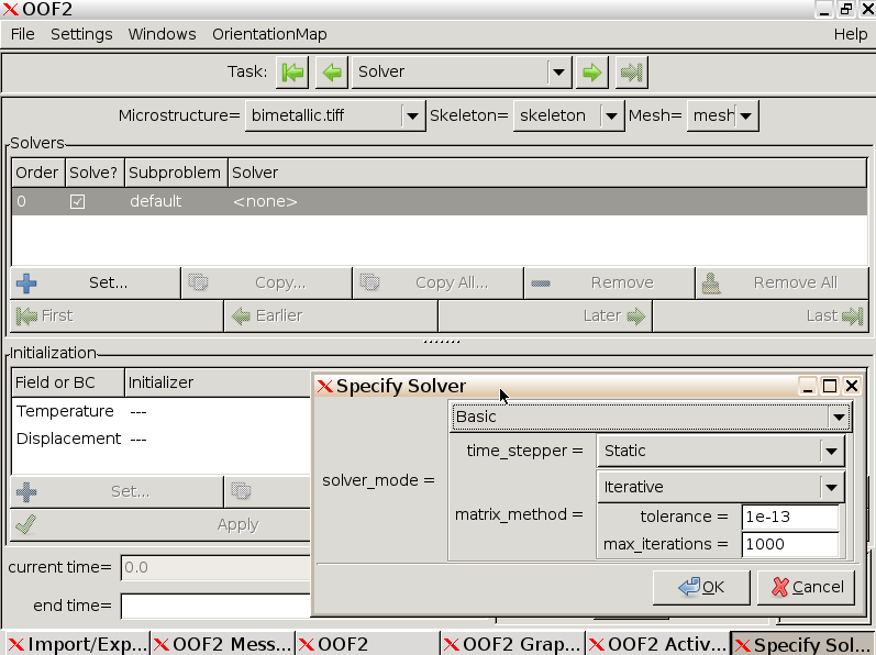
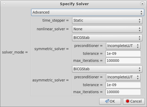
Select the first line in the Solver pane and click “Set…” to specify the solver options. Select “Advanced”, choose BiCGStab (stabilized biconjugate gradient solver) and set tolerance to 1e-9, max_iterations to 100,000 and click OK.
Back in the main pane, click Solve in the bottom right
hand corner to solve the FEM problem. This may take seconds to minutes.
We can watch the progress in the Messages and
Activity windows.
Visualize result. Switch over to the
Graphics window. You will see three layers—the micrograph,
the initial skeleton, and the final mesh.
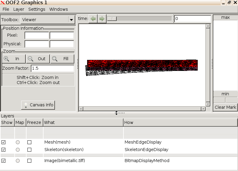
To better visualize the final mesh, uncheck the skeleton in the Layers menu at the bottom of the window.
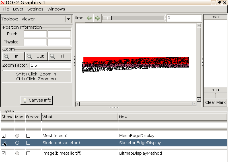
As we may have anticipated, the larger thermal expansion coefficient of the copper relative to the steel has caused the strip to bend downwards under the applied thermal gradient. Depending on the details of your skeleton and mesh, your bimetallic strip may or may not bend as much as this. (In a more detailed study, we should, of course, check how hpr-refinement affects our results.)
We shall now visualize the temperature gradient over the final mesh.
From the Layer dropdown menu, select New.... In the
Displayed Object column on the left, select category
Mesh.
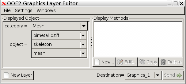
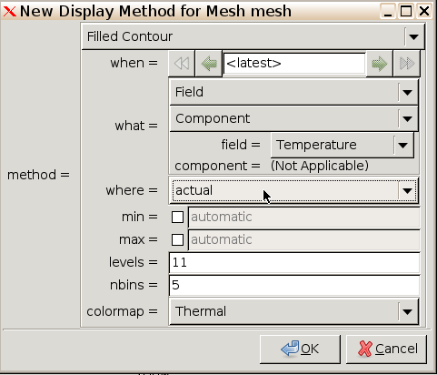
In the Display Methods column on the right, click New...
and select Filled Contour. Specify field to be
Temperature, and where to be actual. Click
OK.
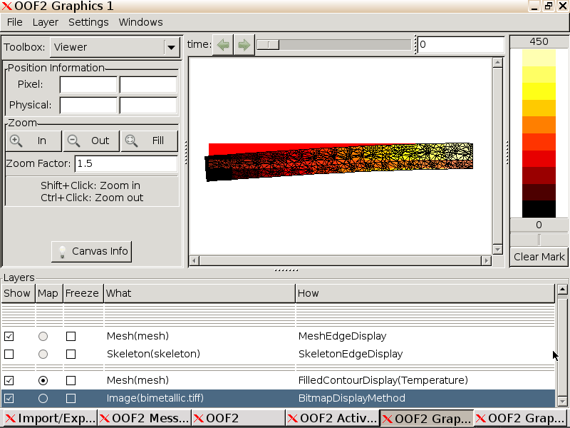
Back in the Graphics window, we now have the terminal temperature gradient overlaid on our final deformed mesh.
Analysis. We will now proceed to extract some
numerical results. In the main OOF2 window, use the Task
dropdown to navigate to the Analysis pane.
Specify in the Output menu, field to be
Temperature, in the Sampling menu, x_points =
10 and y_points = 10, and in the Destination menu the Message Window for
output. (Alternatively, we can write to file by clicking
New... and download the file to our local machine using the
Upload/Download window.) Click Go.
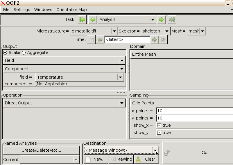
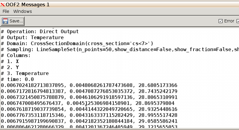
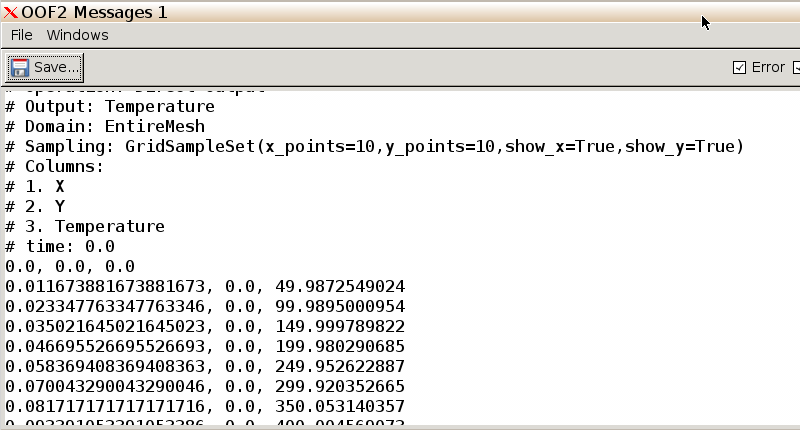
The temperature over a grid is output to the Message
window.
First create a new layer in the same manner as before. In the
Displayed Object column on the left, select category Mesh.
In the Display Methods column, click New... and select
Material Color. Click OK.
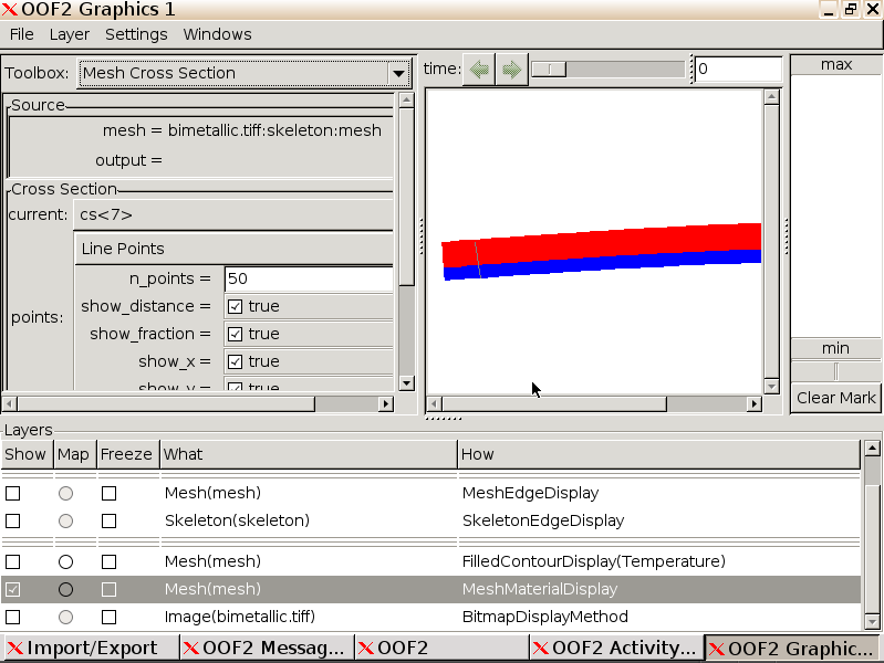
Back in the Graphics window, deselect all Layers except the
MeshMaterialDisplay that we just created. From the Toolbox menu in the
top left, select Mesh Cross Section and then using your
pointer, draw a cross section over the deformed strip. Leave n_points as
50. We will now analyze the temperature at 50 uniformly spaced points
along this line.
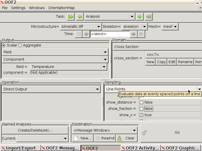
Switch back to the Analysis window. Set field to
temperature, and Domain to Cross Section. Deselect
show_distance and show_fraction since these
are unimportant to us, and leave the Destination as the Message Window.
Click Go.
Checking back in the Message window, we find our results.