How to estimate  ,
,  and
and  of a second order TF with partial data?
estimate the steady state value of the step response of a second order TF with partial data
Contents
% 2016-10-24
% Y\"un Han
% ECE 486 Lab 5

function parmEstimate2ndOrderTF
preamble
clear % clear values of variables in workspace
clc % clear messages in the command window
clf % clear existing figures
close all % close all existing windows; w/o 'all', only close the latest
generate step response with given parameters K, wn and zeta
K - DC gain; wn - natural frequency; zeta - damping ratio;
% choose some K, wn and zeta
K = 3.5;
wn = 10;
zeta = 0.05; % choose low damping so that it takes longer to settle

% we can always generate a unit step response using TF defined by K, wn, zeta
sys = tf(K*wn^2, [1 2*zeta*wn wn^2]);
% obtain the data for step response of the 2nd order TF
Tf = 20; % collect the step response between 0 and Tf
[y, t] = step(sys, 0:0.002:Tf); % UNIT response data
% plot step response
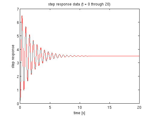
figure(1)
plot(t, y, 'r')
xlabel('time [s]')
ylabel('step response')
title('step response data (t = 0 through 20)')

estimate the full step response graph given partial data from figure 1
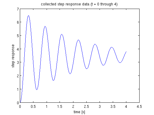
the problem in Lab 5 was, as seen in figure 1, the response was highly oscillatory and when we collected data, we gave a short time window. say in figure 1, we only collected the step response data for a time window 4 sec.
trimIdx = find(t>4, 1, 'first');
figure(2)
plot(t(1:trimIdx),y(1:trimIdx),'b')
xlabel('time [s]')
ylabel('step response')
title('collected step response data (t = 0 through 4)')
% the question is: is it possible to use the graph between t = 0 and t = 4
% to estimate K, wn and zeta of the 2nd order TF such that we can project
% the step response graph from t = 4 on? if possible, we can concatenate
% the projected graph between t = 4 and t = 20, and the data we already got
% between t = 0 and t = 4; the combination of the two would complete the step
% response of a 2nd order TF, i.e.,
% (partial real data + projection = complete response), then you can call your
% script to calculate Mp, tr, ts.

use the data shown in figure 2 as an example, to estimate K, wn and zeta
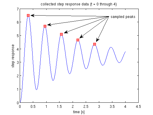
sampled five peak values in figure 2 using data cursor t1 = 0.314; y1 = 6.491; t2 = 0.944; y2 = 5.683; t3 = 1.572; y3 = 5.094; t4 = 2.202; y4 = 4.664; t5 = 2.832; y5 = 4.35;
t1 = 0.314;
y1 = 6.491;
t2 = 0.944;
y2 = 5.683;
t3 = 1.572;
y3 = 5.094;
t4 = 2.202;
y4 = 4.664;
t5 = 2.832;
y5 = 4.35;
tSample = [t1 t2 t3 t4 t5]';
ySample = [y1 y2 y3 y4 y5]';
% show the sample peaks in figure 2
figure(3)
plot(t(1:trimIdx),y(1:trimIdx),'b')
hold on
plot(tSample,ySample,'linestyle','none', ...
    'marker','s','markersize',8, ...
    'markeredgecolor','red','markerfacecolor',[1 0.5 0.5])
% mark down the peaks
annotation('textarrow',[3.2/4.5   0.2],[6/7 ySample(1)/7.5],'string',' ')
annotation('textarrow',[3.2/4.5 0.309],[6/7 ySample(1)/8.3],'string',' ')
annotation('textarrow',[3.2/4.5 0.418],[6/7 ySample(1)/9.1],'string',' sampled peaks')
annotation('textarrow',[3.2/4.5  0.52],[6/7 ySample(1)/9.7],'string',' ')
annotation('textarrow',[3.2/4.5  0.63],[6/7 ySample(1)/10.2],'string','')
xlabel('time [s]')
ylabel('step response')
title('collected step response data (t = 0 through 4)')

% use (t1, y1) through (t5, y5) to estimate K, wn and zeta
% the time domain solution of unit response of second order TF
% y(t)=K*(1-1/sqrt(1-zeta^2)*exp(-zeta*wn*t)*sin(wn*sqrt(1-zeta^2)*t+acos(zeta)))
% --- let's say it is eqn.(+)

% denote damped natural frequence as wd = wn*sqrt(1-zeta^2)
% period is the time difference between adjacent peaks, T = 2*pi/wd
Tavg = mean(diff(tSample));
wd = 2*pi/Tavg; % = wn*sqrt(1-zeta^2), so we know wn times some zeta equals a number

% use data points (t1,y1), (t2,y2), (t3,y3)
% denote M = 1/sqrt(1-zeta^2)*exp(-zeta*wn*t1)*sin(wd*t1+acos(zeta))
%        N = exp(-zeta*wn*T)
% by eqn.(+) above, we have
% y1 - y2 = K*M*N - K*M = K*M*(N-1)         --- eqn.(2)
% similarly,
% y1 - y3 = K*M*N^2 - K*M = K*M*(N-1)*(N+1) --- eqn.(3)
% divide eqn.(3) by eqn.(2), we have
% N + 1 = (y1-y3)/(y1-y2)
% so N = (y1-y3)/(y1-y2) - 1                --- eqn.(N cal.)
% note that N by this method, is independent of M, we can repeat this
% using data points (t2,y2), (t3,y3), (t4,y4)
%                   (t3,y3), (t4,y4), (t5,y5) ...
%                   (t(n),y(n)), (t(n+1),y(n+1)), (t(n+2),y(n+2))

N1 = (y1-y3)/(y1-y2) - 1;
N2 = (y2-y4)/(y2-y3) - 1;
N3 = (y3-y5)/(y3-y4) - 1;
Navg = mean([N1 N2 N3]);
% according to the notation of N
% now we have
% zeta*wn = -log(N)/T
% also by notation of wd
% sqrt(1-zeta^2)*wn = 2*pi/T

% solve for wn and zeta by using N and T
% we need to call numerical solver fsolve for a system of nonlinear
% equations
% note: you need Optimisation Toolbox in order to use fsolve
x0 = [.5; 2];  % init guess for zeta and wn
% call solver; check funcWnZetaVal, it should be almost 0
% parmSolve2ndOrderTF is defined below
if (strcmp(version,'7.14.0.739 (R2012a)'))
    options = optimset('Display','iter'); % for the older matlab
else
    options = optimoptions('fsolve','Display','iter'); % display iteration output
end
[x,funcWnZetaVal] = fsolve(@(x)parmSolve2ndOrderTF(x,Navg,Tavg),x0,options)


zetaEst = x(1) % compare our estimation with the acutal zeta = 0.05
wnEst = x(2) % compare with the actual wn = 10

% how about K, the steady state value - the most important parameter we
% care about? K = y1/(1-M) etc
K1 = y1/(1-MCal(zetaEst,wnEst,t1)); % Mcal is defined below
K2 = y2/(1-MCal(zetaEst,wnEst,t2));
K3 = y3/(1-MCal(zetaEst,wnEst,t3));
KEst = mean([K1 K2 K3]) % compare with the actual K = 3.5

% estimation success!
                                         Norm of      First-order   Trust-region
 Iteration  Func-count     f(x)          step         optimality    radius
     0          3         68.2985                          10.5               1
     1          6         59.3283              1           10.4               1
     2          9         54.5859              1           16.4               1
     3         12         51.7324              1           18.4               1
     4         15         48.6071              1           20.7               1
     5         18         46.9557              1           21.8               1
     6         21          44.497              1           23.6               1
     7         22          44.497              1           23.6               1
     8         25         35.8988           0.25           10.2            0.25
     9         28         32.2251           0.25           5.68            0.25
    10         31         29.4594           0.25           5.43            0.25
    11         34         23.1886          0.625           4.79           0.625
    12         37         16.3753         1.5625           19.8            1.56
    13         40         4.54797         1.5625           10.9            1.56
    14         43        0.115856         1.5625           2.59            1.56
    15         46     4.79918e-05       0.216091         0.0598            3.91
    16         49     7.21531e-12     0.00354632          2e-05            3.91
    17         52     1.68422e-25    1.80101e-06       3.66e-12            3.91

Equation solved.

fsolve completed because the vector of function values is near zero
as measured by the default value of the function tolerance, and
the problem appears regular as measured by the gradient.


x =

    0.0501
    9.9938


funcWnZetaVal =

   1.0e-12 *

    0.3559
   -0.2043


zetaEst =

    0.0501


wnEst =

    9.9938


KEst =

    3.5009

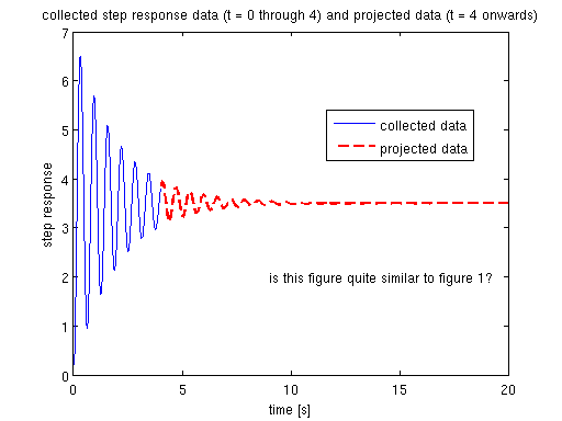
complete the partial plot with our projection
figure(4)
% create the projected TF for from t = 4 sec onwards
sysProj = tf(KEst*wnEst^2, [1 2*zetaEst*wnEst wnEst^2]);
% projected response data
[yProj, tProj] = step(sysProj, 0:0.002:Tf); % UNIT response data
% plot both collected data (blue) and projected data (red)
plot(t(1:trimIdx),y(1:trimIdx),'b','linewidth',1.5)
hold on
plot(tProj(trimIdx:end),yProj(trimIdx:end),'r--','linewidth',2)
xlabel('time [s]')
ylabel('step response')
legend('collected data','projected data','location','best')
text(9,2,'is this figure quite similar to figure 1?')
title('collected step response data (t = 0 through 4) and projected data (t = 4 onwards)')

end % parmEstimate2ndOrderTF

function funcWnZeta = parmSolve2ndOrderTF(x,N,T)
    % x = (zeta, wn)
    funcWnZeta = [x(1)*x(2) + log(N)/T;
                  sqrt(1-x(1)^2)*x(2) - 2*pi/T];
end

function M = MCal(zeta,wn,t)
    M = 1/sqrt(1-zeta^2)*exp(-zeta*wn*t)*sin(wn*sqrt(1-zeta^2)*t+acos(zeta));
end