 |
CS440/ECE448 Spring 2020Assignment 6: Neural Nets and PyTorchDue date: Wednesday April 22th, 11:59pm |
Created By: Justin Lizama, Kuangxiao Gu and Yuqian Zhou
The goal of this assignment is to get some hands on experience with neural networks. The dataset used in this MP is fashionMNIST, where the dataset consists of grayscale images of size 28*28 containing different type of clothes. In part 1, you will create a simple fully connected neural network to classify cloth, shoes and bags. In part 2, the goal is to do a classification between different type of clothes, which is a harder task than the first part due to the similarity between those clothes. For extra credit, the goal is to implement a simple autoencoder for image reconstruction task.
You will be using the PyTorch and NumPy library to implement these models. The PyTorch library will do most of the heavy lifting for you, but it is still up to you to implement the right high level instructions to train the model.
For the entire MP6, please use CPU for training. Please DON'T change the provided parameter list in code template. The train/dev data will be provided as torch.tensor; please divide them into batches manually without using PyTorch dataLoader.
Contents
- Dataset
- Part 1: Simple Fully-connected Networks
- Part 2: Modern Networks
- Extra Credit
- Provided Code Skeleton
- Deliverables
Dataset
The data set can be downloaded here: data (gzip) or data (zip). When you uncompress this you'll find a set of *.npy files of format (X,y)_(train,dev)_(part1,part2).npy. The reader.py will load them for you.
Part 1: Simple fully-connected network
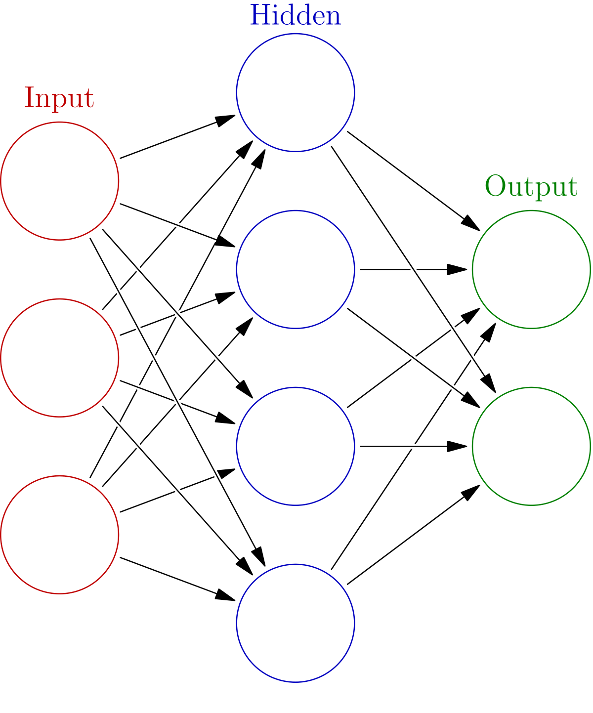
The basic neural network model consists of a sequence of hidden layers sandwiched by an input and output layer. Input is fed into it from the input layer and the data is passed through the hidden layers and out to the output layer. Induced by every neural network is a function \(F_{W}\) which is given by propagating the data through the layers.Training and Development
- Training: To train the neural network you are going to need to minimize the empirical risk \(\mathcal{R}(W)\) which is defined as the mean loss determined by some loss function. For this assignment you can use cross entropy for that loss function: \[ \mathcal{R}(W) = \frac{1}{n}\sum_{i=1}^n\sum_{c=1}^C I(y_i=c) \log \hat y_i^c . \] Where the \(y_i\) are the labels. \(I(y_i=c)\) is a indicator function which takes value 1 when \(y_i=c\) and 0 otherwise. \(\hat y_i^c\) is the network output for datapoint i and class c. The \(\hat y_i \) are determined by \(\hat y_i = softmax(F_{W}(x_i))\). For this assignment, you won't have to really implement this yourself. You can just use the PyTorch function torch.nn.CrossEntropyLoss(). Although the final probability for each class, mathmatically, should be \(\hat y_i = softmax(F_{W}(x_i))\), notice that torch.nn.CrossEntropyLoss() functions expects raw input without normalization. As a result, do not apply any activation function to the last layer of your network.
- Development: After you have trained your neural network model, you will have your model classify each image as either cloth, shoes or bags with labels 0,1,2, respectively. This is done by evaluating your network on each example in the development set, and then taking the index of the maximum of the three outputs (i.e. argmax).
Part 2: Modern Network
In this part, you will try to perform a harder classification task with 5 classes, with modern neural network techniques. These include, but are not limited to the following:- Choice of activation function: Some possible candidates are (Tanh, ReLU, SELU, and LeakyReLU). You may find that choosing the right activation function will lead to faster convergence, and or improved performance overall.
- L2 Regularization: Regularization is when you try to improve your model's ability to generalize to unseen examples. One commonly used form of regularization is L2 regularization. Let \(\mathcal{R}(W)\) be the empirical risk (mean loss), then you can implement L2 regularization by adding on an additional term that penalizes the norm of the weights. More precisely, your new empirical risk becomes \(\mathcal{R}(W):= \mathcal{R}(W) + \lambda \sum_{W \in P} \Vert W \Vert_2 ^2\) where \(P\) is the set of all your parameters and \(\lambda\) (usually small) is some hyperparameter chosen by you.
- Network Depth and Width: The sort of network you implemented in part 1 is called a two-layer network because it uses two weight matrices. Sometimes it helps performance to add more hidden units and/or add more weight matrices to obtain greater representation power and make training easier.
- Data Standardization (Recommanded): Convergence speed can be improved greatly by simply centralizing your data by subtracting the sample mean and dividing by the sample standard deviation. More precisely, you can alter your data matrix \(X\) by simply doing \(X:=(X-\mu)/\sigma\).
- Consider using convoluiton 2D layers as 1st layer, the channel size could be 16 with kernel size 3, stride 1 and padding 1. MaxPooling layers is optional after conv2d layer.
Same as part 1, do not apply any activation function to your final layer.
Try to employ some of these techniques in order to attain a test accuracy of at least 0.73 while keeping the total number of parameters under 500,000. This means that if you take every floating point value in all of your weights including bias terms, you only use at most 500,000 floating point values.Extra Credit
Note that for this part, the input to fit() function will be provided with shape [number of datapoints, 784] as before, which means you need to change it to image shape format of [batch_size, 1, 28, 28] in order to feed it into your encoder.
Try to get a MSE less than 0.03 in this part.
Here is a simple autoencoder tutorial just for reference: https://medium.com/@vaibhaw.vipul/building-autoencoder-in-pytorch-34052d1d280c
Provided Code Skeleton
We have provided ( tar zip) all the code to get you started on your MP, which means you will only have to implement the PyTorch neural network model. There was previously a typo on the train_set shape, which should be [N, 784]. The current template code fixed that typo.
- reader.py - This file is responsible for reading in the data set.
- mp6.py - This is the main file that starts the program, and computes the accuracy, precision, recall, and F1-score using your implementation.
- neuralnet_(p1, p2, p3).py These are the files where you will be doing all of your work for each part. You are given a NeuralNet class which implements a torch.nn.module. This class consists of __init__(), set_parameters(), get_parameters(), forward(), and step() functions.
In the __init__() function you will need to construct the network architecture. There are multiple ways to do this. One way is to use nn.Linear() and nn.Sequential() . Keep in mind that nn.Linear() uses a Kaiming He uniform initialization to initialize the weight matrices and 0 for the bias terms. Another way you could do things is by explicitly defining weight matrices W1,W2,... and bias terms b1,b2,... by defining them as a torch.tensor(). This way is more hands on and will allow you to choose your own initialization. However, for this assignment Kaiming He uniform initialization should suffice and should be a good choice. Additionally, you can initialize a torch.optim optimizer object in this function to use to optimize your network in the step() function.
The forward() function should do a forward pass through your network. This means it should explicitly evaluate \(\sigma (F_{W}(x))\) . This can be done by simply calling your nn.Sequential() object defined in __init__() or in the torch.tensor() case by explicitly multiplying the weight matrices by your data.
The step() function should perform one iteration of training. (One iteration means processing one batch, not the entire training dataset, which is usually called an epoch). This means it should perform one gradient update through your current batch training data. You can do this by calling loss_fn(yhat,y).backward(), then either updating the weights directly yourself, or you can use a torch.optim object that you may have initialized in __init__() to help you update the network. Be sure to call zero_grad() on your optimizer in order to clear the gradient buffer.
More details on what each of these methods in the NeuralNet class should do is given in the skeleton code.
The function fit() takes as input the training data, training labels, development set, and maximum number of iterations. The training data provided is the output from reader.py. The training labels is a torch tensor consisting of labels corresponding to each image in the training data. The development set is the torch tensor of images that you are going to test your implementation on. The maximum number of iterations is the number you specified with --max_iter (by default it is set to 50). For part 1, the mp6.py and autograder will run your training for max_iter iterations. For part 2 and extra credit, mp6.py and autograder will run your training for 2*max_iter iterations. fit() outputs the predicted labels. The fit function should construct a NeuralNet object, and iteratively call the neural net's step() function to train the network. This should be done by feeding in batches of data determined by batch size. (You will use a batch size of 100 for this assignment.). If you need to change the input shape to your neural net, please perform this operation in the forward() function in NeuralNet class (instead of in fit() function)
Do not modify the provided code. You will only have to modify neuralnet_(p1, p2, p3).py.
To understand more about how to run the MP, run python3 mp6.py -h in your terminal.
Definitely use the PyTorch docs to help you with implementation details. You can also use this PyTorch Tutorial as a reference to help you with your implementation. There are also other guides out there such as this one.
Deliverables