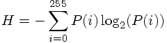
Given babooon.png and lena.png, modify the skeleton code for Part 1 to compute
of each image, where P(i) the probability that a pixel has intensity value i.
The following points are important:
In the skeleton source code given to you, the histogram is already computed. In order to find the entropy, you have to find the probabilities from the histogram. This is done by normalization. You simply divide each element of the histogram array by the total number of pixels of the image to do this normalization.
Once you find the probabilities, apply the formula at the top given above to compute the entropy.
Entropy is a very important concept in image compression. It is a crude measure of the average number of bits that is spent to code each pixel (or symbol in general, if you are interested and want to learn more about entropy, consult Information Theory books, though it is completely unnecessary for this class).
When you compute the entropy, be careful about the integer division properties of C++. That is why you should convert the types to doubles or floats before you carry out division.
Note that some values will have zero probability, these are the ones which do not occur in the image. For these ones, if you use the value of 0log2(code), you will get NaN as a result. Therefore, whenever you come across a zero probability value, use the following convention 0log2(0)=0. This is provided in the log2 funcion in the skeleton code.
Make sure your code outputs the histogram values into a file, and displays the entropy and total number bits on the screen.
Run length coding is a very common lossless compression technique. Details about this method will be explained in the lab session by some examples. Modify the skeleton code to compute the run length code of lenaerrdiff.png and weaskedforit.png.
The following points are important:
In the skeleton code that is given to you, the routine is prepared such that the values are scanned in the so-called "raster-snake" order. This methodology will also be explained in the lab session. Do not modify the scanning order in the skeleton code that is given to you.
Both images that you are going to experiment with in this part are binary valued images. But the pixels of these images take the values of 0 and 255. The skeleton code is prepared such that this is scaled to have the values of 0 and 1 only.
Given the binary images, you are going to find the "run-lengths". Then you are going to find the histogram that corresponds to these run-lengths. In the end you will find the entropy from this histogram, hence this entropy is going to correspond to the bit rate that is going to be spent to code each run on average. Do not forget to scale this histogram by the total number of runs to find the probabilities (recall the argument in Part 1). Once you find the probabilities, you can easily find the entropy from these.
In this code, you are going to write the histogram values to a file. Note that you will write the histogram values of the run-lengths, not the histogram of the original pixels. When you write these values to a file, you can use a similar routine that is given in part 1 above.
You are also going to display the entropy on the screen. The entropy here is a measure of bits/run. You are also going to display the total number of bits, which is (entropy)*(total number of runs) and the average number of bits that is going to be spent per pixel on the screen. Observe that this average number of bits is expressed by (total number of bits)/(number of pixels).
Make sure your code outputs the run length histogram values into a file, and displays entropy, total number of bits and bits spent per pixel on the screen.
Compile lab10-bitplanes.cc (without modification) using
gmake lab10-bitplanes
This command will produce the executable file bitplanes. This file seperates a given a grayscale image into 8 different images, which are all bilevel. These images are called the bitplanes of the original image. The conversion from the grayscale value to the individual bitplanes is done by first mapping the binary digits of the grayscale value to gray-coded binary values so as to minimize the number of bitplanes whose values will change due to a small change in the value of the intensity value. This point will be explained further during the lab-session. An example usage of this function would be:
./lab10-bitplanes lena.png lena_bit
After execution, 8 images will be produced, with the names:
lena_bit0.png

lena_bit1.png

lena_bit2.png

lena_bit3.png

lena_bit4.png

lena_bit5.png

lena_bit6.png

lena_bit7.png
All of these images are composed of the pixel values 0 or 255, from the bit planes of lena.png. You are going to process these bit plane images using the code of part 2. There is no seperate code needed for this part.
Form 8 binary versions of lena.png, one for each bit plane, using the executable file lab10-bitplanes. Now use your code from Part 2 to run length code each of the 8 bit plane images of lena. Observe that the least significant bit plane is the noisiest bit plane.
For each bit plane, make sure your code outputs the run length histogram values into a file, and outputs the entropy value (bits/run), the total number of bits and the average number of bits spent/pixel on the screen (as you did in Part 2).
In this part you will do predictive coding. The following points are important:
In this part you may assume the image will be 512*512 pixels.
Go through the image in "raster snake order" (I will explain this during lab), and assume that a pixel's intensity value will very likely be the same as its previous neighbor's intensity value. A loop that goes through the pixels in this order is already provided for you. You will simply predict the current pixel's value from its causal neighbor. By using this prediction idea, you will find the differences between the original pixel and its predicted value. Note that there are going to be a total of (512*512-1) difference values since there are a total of (512*512) pixels. This methodology is motivated by the fact that you expect the current pixel value to be very close to its neighbor value since natural images have pretty smooth characteristics most of the time.
Find the histogram of the difference pixel values using the same ideas in Part 1 of this lab. Note the important difference that, your difference pixel values can potentially have values in the range -255,-254,...,-1,0,1,..,254,255 (whereas the original image pixels take values in the range of 0,1,...,254,255). Therefore the histogram vector histogram is going to be of size 511 (this array was of size 256 in Part 1).
Using the same ideas as in Part 1, find the entropy of these difference pixel values. Do not forget to normalize the histogram values by the total number of difference pixels which is 512*512-1. This normalization is crucial in entropy computation.
Finally store the histogram values of the difference pixels in a file. Also display the entropy and the total number of bits on the screen (This time total number of bits is equal to the product of entropy and 512*512-1).
Carry out the experiments in Part 4 for both lena.png and baboon.png images. Compare the entropy values you found in this part with the entropy values you found in Part 1 for each image. This gives you some hints about the usage of predictive coding in lossless compression.