Min Cut and Max Cut
Random contraction and random hyperplanes · Lecture 24 · November 13, 2026
Sariel Har-Peled
CS 574 · University of Illinois, Urbana-Champaign
One graph, two optimization problems
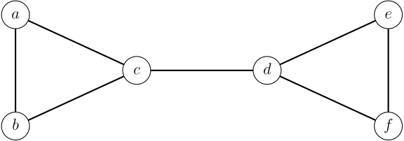
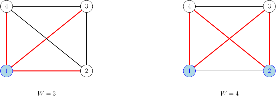
Partition the vertices into two nonempty sets.
How few edges can cross? How many can cross?
Ask for both answers before advancing. Minimum 1; maximum 5. Use the same graph throughout the contraction examples. All graphs in the min-cut part are undirected and unweighted; contraction produces integer multiplicities.
Today’s route
Minimum cut
Contract a random edge
25
Faster minimum cut
Branch before contraction gets risky
15
Maximum cut
Round vectors with a random hyperplane
25
Why the relaxation is convex
Use a Gram matrix
10
Min cut: preserve one optimal solution.
Max cut: preserve a fraction of the relaxed objective in expectation.
A cut is a partition
For \(G=(V,E)\) , write \(n=|V|\) and \(m=|E|\) .
For \(\varnothing\ne S\subsetneq V\) , define
\[\delta(S)=\{uv\in E:u\in S,\ v\notin S\}.\]
The cut size is \(|\delta(S)|\) .
\(S\) and \(V\setminus S\) describe the same cut.
We begin with a connected graph; a disconnected graph has min cut \(0\) .
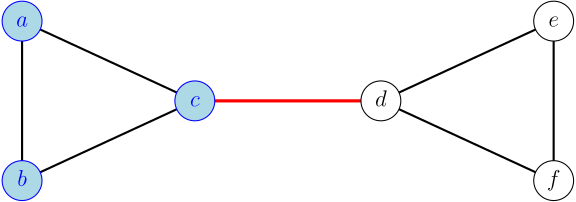
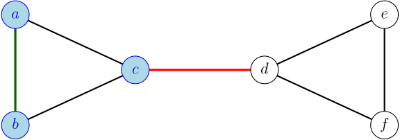
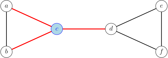
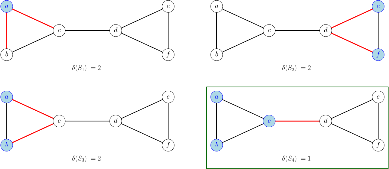
The smallest cut in our example
\[S=\{a,b,c\},\qquad |\delta(S)|=1.\]
The bridge \(cd\) is a minimum cut.
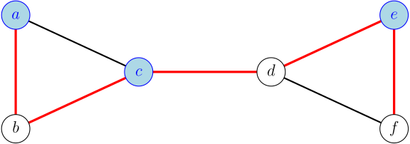
The largest cut in the same graph
\[S=\{a,c,e\},\qquad |\delta(S)|=5.\]
Each triangle contributes at most two edges; the bridge contributes at most one.
Min cut: shrink the graph
Choose an edge \(uv\) and merge its endpoints into one supervertex .
Delete self-loops. Keep parallel edges.
Each supervertex remembers the original vertices it contains.
Stop when two supervertices remain: they define a cut of the original graph.
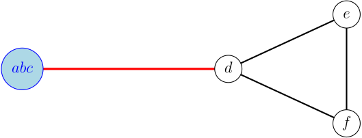
Choose an edge inside one side
Contract \(ab\) . The target cut keeps \(a\) and \(b\) together anyway.
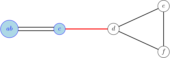
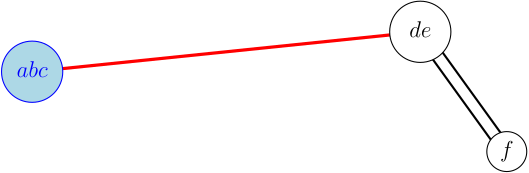
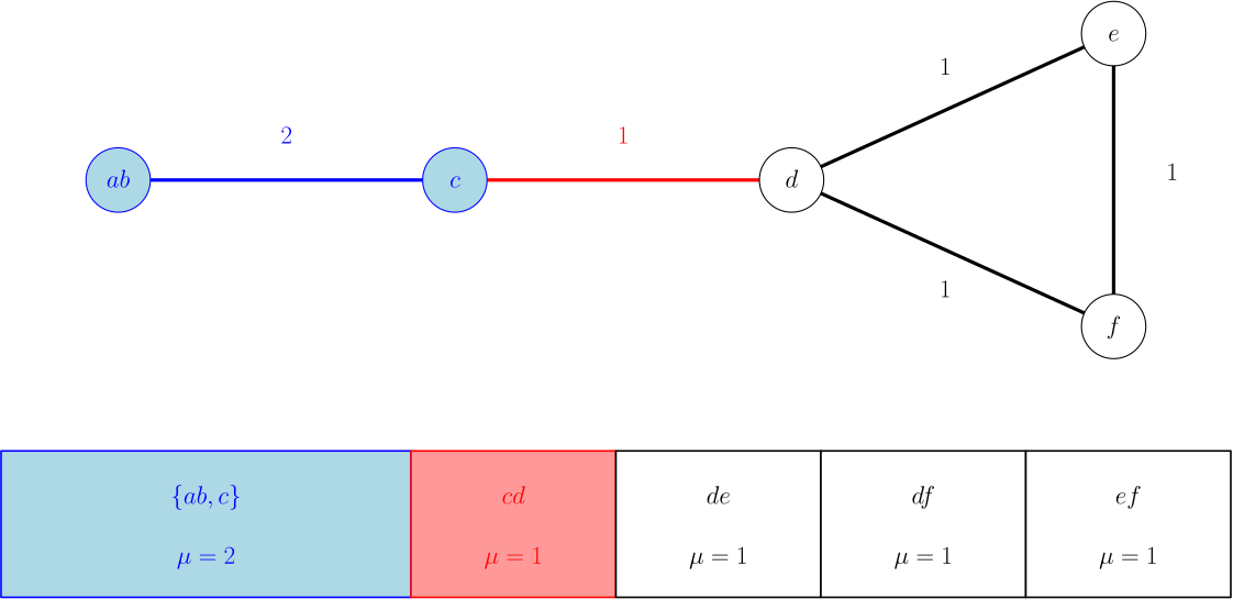
Parallel edges are essential
The two edges represent the original edges \(ac\) and \(bc\) .
Sample uniformly among edge copies , including multiplicities.
There are six remaining edge copies. The pair (ab,c) must be selected with probability 2/6, not 1/5. A weighted representation of multiplicities must sample proportionally to the integer weight.
Finish the left triangle
Contract one of the two edges between \(ab\) and \(c\) .
Both copies become self-loops and disappear. The bridge survives.
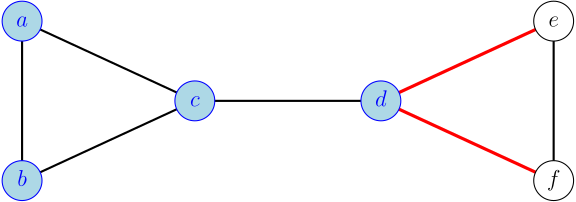
Shrink the right side
The target cut still has one crossing edge.
Two supervertices give the answer
\[\{a,b,c\}\ \mid\ \{d,e,f\}.\]
Count the remaining edge copies: the returned cut has size \(1\) .
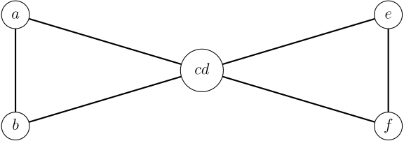
What if we contract the bridge?
No later cut can put \(c\) and \(d\) on opposite sides.
The original bridge cut has been lost.
A valid answer can still be suboptimal
Contracting \(cd\) , then \(ab\) , then \(ef\) , then \(ab\) with \(cd\) can return
\[\{a,b,c,d\}\mid\{e,f\},\qquad |\delta(S)|=2.\]
What contraction preserves
Every cut of a contracted graph lifts to a cut of the original graph, with the same size .
Contraction can remove candidate cuts. It cannot create a smaller cut.
Fix one minimum cut \(C\) . If no contracted edge belongs to \(C\) , then \(C\) survives.
The fixed-cut event is sufficient for success. Destroying one minimum cut need not destroy all minimum cuts. Our bridge example has a unique minimum cut, so contracting its bridge really does rule out every optimum.
Karger’s random contraction algorithm
Start with one supervertex per original vertex.
While more than two remain, choose a uniformly random edge copy and contract it.
Delete self-loops and retain all other edge copies.
Return the cut defined by the final two supervertices.
We never need to know which edges belong to a minimum cut.
A small cut forces many safe edges
Let the minimum cut have size \(k\) .
Every vertex has degree at least \(k\) , because isolating it gives a cut.
Therefore
\[2m=\sum_{v\in V}\deg(v)\geq nk,\qquad m\geq\frac{nk}{2}.\]
Only \(k\) of these edge copies belong to the fixed cut \(C\) .
The next contraction is unlikely to hit C
Condition on \(C\) surviving until \(r\) supervertices remain.
The current graph still has minimum cut \(k\) , so
\[\Pr[\text{contract an edge of }C\mid C\text{ survives}]
=\frac{k}{m_r}\leq\frac{2}{r}.\]
The chance of a safe next step is at least \(1-2/r\) .
The surviving cut supplies an upper bound k on the contracted min cut; lifting supplies the lower bound k. Degrees and m_r count multiplicities. On our six-vertex graph the first-step failure probability is 1/7; 2/6 is only an upper bound.
Multiply conditional probabilities
\[\begin{aligned}
\Pr[C\text{ survives to two vertices}]
&\geq\prod_{r=3}^{n}\left(1-\frac2r\right)\\
&=\frac{n-2}{n}\frac{n-3}{n-1}\cdots\frac13\\
&=\boxed{\frac{2}{n(n-1)}}.
\end{aligned}\]
The contraction events are dependent. The chain rule is enough.
Repeat and keep the smallest cut
Let \(p=2/[n(n-1)]\) and run \(R\) independent trials.
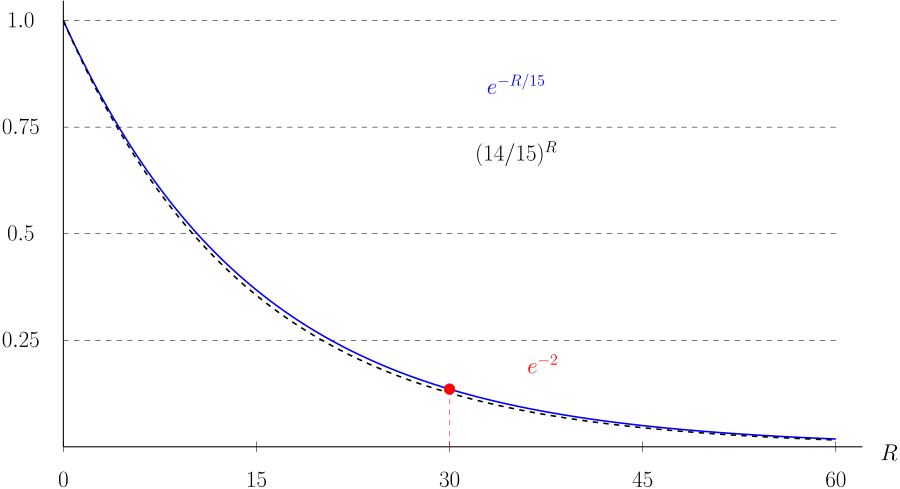
\[\Pr[\text{all trials fail}]\leq(1-p)^R\leq e^{-pR}.\]
For \(R=n(n-1)\) , failure is at most \(e^{-2}<0.14\) .
Keeping the smallest returned cut is safe: no trial can return less than optimum.
Cost of the basic algorithm
With a multiplicity representation, one contraction takes \(O(n)\) time.
One trial: \(O(n^2)\) .
Constant success probability: \(O(n^4)\) .
High probability: \(O(n^4\log n)\) .
The notes also give a random-weight MST interpretation.
For example, maintain an adjacency matrix of multiplicities, vertex degrees, and weighted sampling structures. Sample a vertex proportional to degree and then a neighbor proportional to multiplicity. Merging rows/columns and maintaining degrees takes O(n). The notes’ MST variant assigns independent continuous random priorities, runs Kruskal, and deletes the largest-priority MST edge. A linear-time bottleneck-partition implementation is an exercise in the source, not proved here.
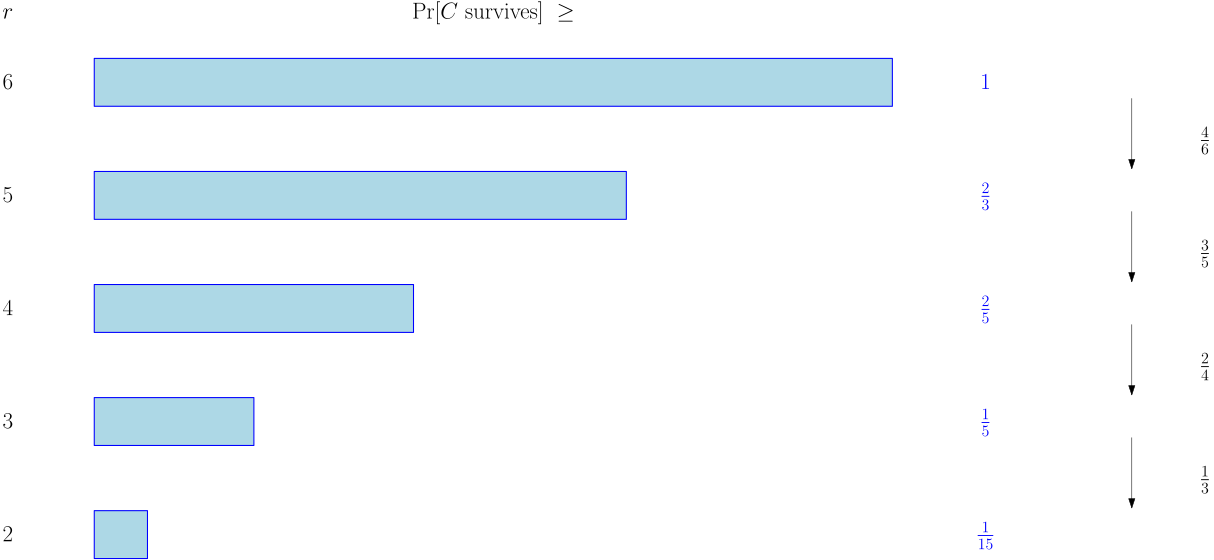
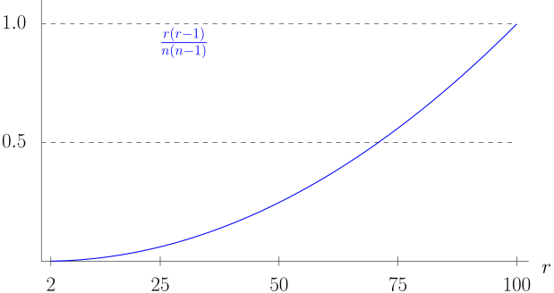
The risky steps come late
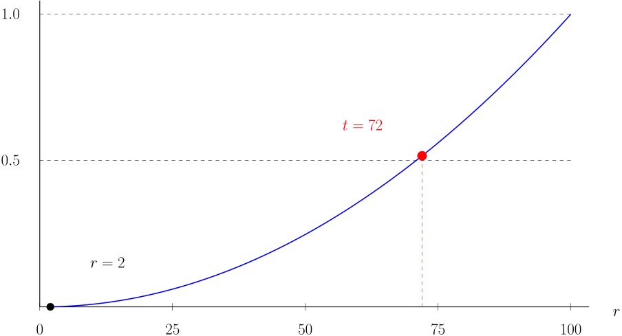
\[\Pr[C\text{ survives down to }r]\geq\frac{r(r-1)}{n(n-1)}.\]
Read the curve from right to left as contraction proceeds.
Branch before the graph gets too small
Share the cheap, safer progress. Spend repetitions near the risky end.
Karger–Stein: FastCut
If \(n\leq6\) , enumerate all cuts and return a minimum cut.
Otherwise set \(t=\lceil1+n/\sqrt2\rceil\) .
Independently contract two copies of \(G\) to \(t\) vertices.
Recursively solve both smaller graphs; return the smaller lifted cut.
The two branches use independent random choices.
Each branch preserves C with probability at least 1/2
\[\Pr[C\text{ survives to }t]\geq\frac{t(t-1)}{n(n-1)}\geq\frac12,\]
where \(t=\lceil1+n/\sqrt2\rceil\) .
The \(+1\) and ceiling make the finite-\(n\) inequality valid.
One surviving branch is enough, provided its recursive call succeeds.
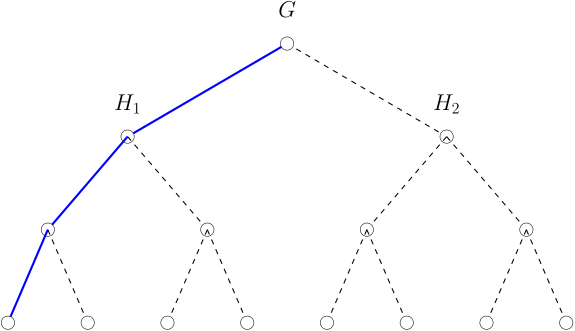
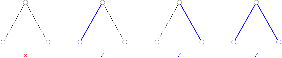
A binary-tree survival experiment
In a complete binary tree of height \(h\) , independently retain each edge with probability \(1/2\) .
Let \(\rho_h\) be the probability of a retained root-to-leaf path; \(\rho_0=1\) .
This is the notes’ black/white edge experiment, drawn with a blue path and dashed supporting edges for readability. It is a comparison process. Actual contraction events are not independent fair coins across the entire recursion tree; the next slides use a conditional lower-bound recurrence.
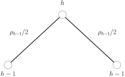
The branching recurrence
\[\rho_h=1-\left(1-\frac{\rho_{h-1}}2\right)^2
=\rho_{h-1}-\frac{\rho_{h-1}^2}{4}.\]
For height one, \(\rho_1=1-(1/2)^2=3/4\) .
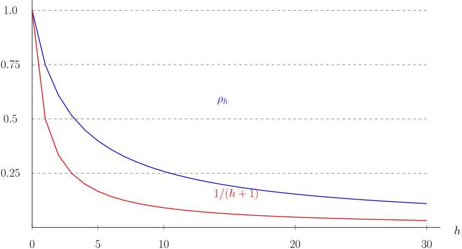
Survival is at least inverse depth
\[\boxed{\rho_h\geq\frac1{h+1}}.\]
For \(f(x)=x-x^2/4\) , \(f\) is increasing on \([0,1]\) .
If \(\rho_{h-1}\geq1/h\) , then
\[\rho_h\geq\frac1h-\frac1{4h^2}\geq\frac1{h+1}.\]
The final inequality is equivalent to \(3h\geq1\) ; the base case is \(h=0\) .
Apply the comparison to FastCut
Let \(p_h\) be a uniform success lower bound for calls with at most \(h\) levels left.
Each branch succeeds with probability at least \(p_{h-1}/2\) .
Conditional on the input graph, the two branches are independent, so
\[p_h\geq1-(1-p_{h-1}/2)^2\geq\rho_h.\]
Depth \(h=O(\log n)\) gives success probability \(\Omega(1/\log n)\) .
At each call fix any minimum cut of that input graph. Conditional on preserving it, the child still has the same optimum, and the uniform recursive guarantee applies. This avoids falsely asserting that all actual preservation indicators are independent Bernoulli(1/2). Exact base cases have success 1; shallow branches can be padded in the comparison process.
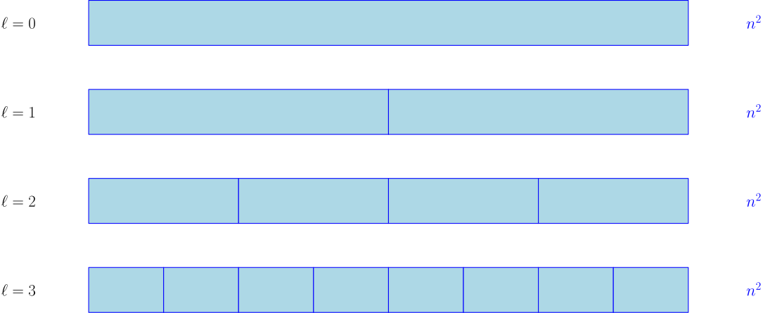
Work at each recursion level
Ignoring bounded rounding terms,
\[T(n)=2T(n/\sqrt2)+O(n^2).\]
At level \(\ell\) :
\[2^\ell\cdot O\!\left((n/\sqrt{2^\ell})^2\right)=O(n^2).\]
There are \(O(\log n)\) levels: one FastCut run costs \(O(n^2\log n)\) .
Amplify the faster algorithm
One run succeeds with probability at least \(c/\log n\) for a constant \(c>0\) .
After \(R=O(\log^2 n)\) independent runs,
\[\Pr[\text{failure}]\leq e^{-cR/\log n}\leq n^{-2}.\]
Total time: \(\boxed{O(n^2\log^3 n)}\) .
Again, return the smallest cut found.
Check the min-cut proof
Why must parallel edges retain their multiplicities?
Why can the min cut never decrease under contraction?
Why is preserving one fixed minimum cut enough?
Pause about one minute. Answers: multiplicities determine both cut values and uniform edge-copy sampling; every contracted cut lifts with the same value; if the fixed cut survives to two supervertices, their partition is optimal. With several minima, other cuts may also survive.
Switch objectives: maximize the crossing weight
For each edge \(ij\) , let \(\omega_{ij}\geq0\) ; set \(\omega_{ij}=0\) on nonedges.
\[\operatorname{OPT}=\max_{S\subseteq V}\;
\sum_{i\in S,\ j\notin S}\omega_{ij}.\]
MAX CUT is NP-hard. We seek an approximation.
Nonnegative weights will be essential when summing edgewise inequalities.
A weighted example
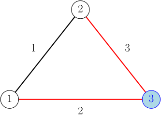
\[w(\{3\},\{1,2\})=2+3=5.\]
Every cut of a triangle misses an edge; missing the lightest is optimal.
Encode the cut by signs
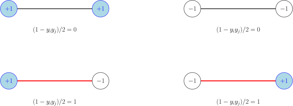
Assign \(y_i=+1\) for \(i\in S\) and \(y_i=-1\) otherwise.
\[\frac{1-y_i y_j}{2}=
\begin{cases}
0,&y_i=y_j,\\
1,&y_i\ne y_j.
\end{cases}\]
\[\operatorname{OPT}=\max_{y_i\in\{-1,+1\}}
\frac12\sum_{i<j}\omega_{ij}(1-y_i y_j).\]
A triangle cannot satisfy every edge
If \(y_1\ne y_2\) and \(y_2\ne y_3\) , then \(y_1=y_3\) .
The edge preferences are coupled by a single assignment to every vertex.
Relax signs to unit vectors
Replace \(y_i\in\{-1,+1\}\) by a unit vector \(v_i\) :
\[\gamma^*=\max_{\|v_i\|=1}
\frac12\sum_{i<j}\omega_{ij}(1-\langle v_i,v_j\rangle).\]
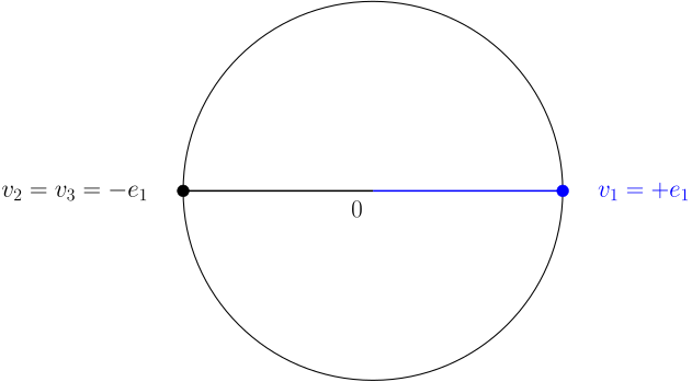
A sign assignment is feasible: choose \(v_i=y_i e_1\) .
Therefore \(\gamma^*\geq\operatorname{OPT}\) .
The source uses the unit sphere in R^(n+1); a Gram representation in R^n already suffices for n vectors. We leave the ambient dimension implicit until the matrix slides. The vector parameterization is not itself a convex feasible region; the Gram-matrix formulation is convex.
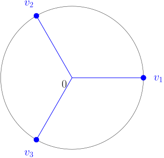
Vectors can spread around a triangle
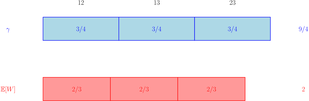
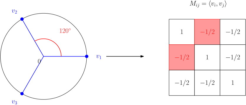
Each pair has dot product \(-1/2\) , hence contribution \((1+1/2)/2=3/4\) .
The relaxed value is \(3\cdot3/4=9/4\) , while \(\operatorname{OPT}=2\) .
This is an optimal vector solution: ||v1+v2+v3||² >= 0 implies the sum of pairwise dot products is at least -3/2, giving objective at most 9/4. Equality holds for the three equally spaced vectors. This calculation is a concrete specialization of the source relaxation.
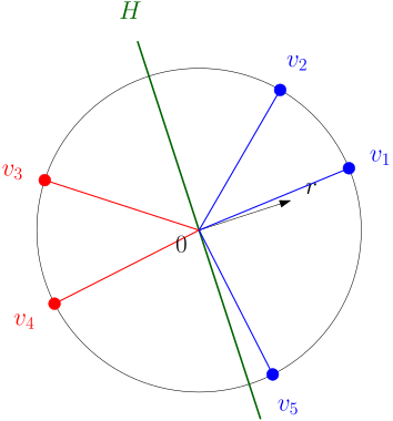
Round with a random hyperplane
Compute a nearly optimal feasible vector solution.
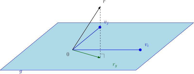
Choose a uniform random unit normal \(r\) .
Set \(S=\{i:\langle v_i,r\rangle\geq0\}\) .
The boundary is the hyperplane \(H=\{x:\langle x,r\rangle=0\}\) .
Both endpoints use the same random normal.
Membership is a set of vertex indices, correcting the source’s shorthand set of vectors. Zero dot products have probability zero for a fixed finite collection of unit vectors. The rounding algorithm may give a trivial zero-weight partition; if a nontrivial partition is required, replacing it by any nontrivial cut cannot reduce its weight because all weights are nonnegative.
A concrete hyperplane cut
This picture shows a planar vector configuration. The algorithm also works in higher dimensions.
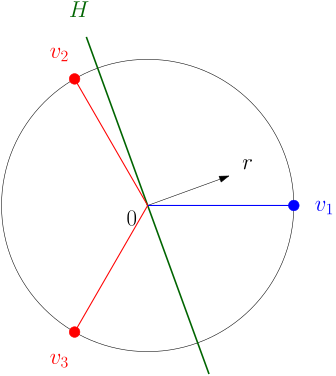
Round the triangle
The cut is \(\{1\}\mid\{2,3\}\) and has weight \(2\) .
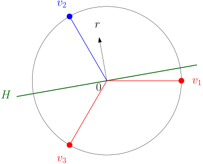
Rotate the normal
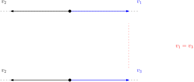
Every nonboundary normal yields a \(1\) –\(2\) split of these three vectors.
Rounding returns weight \(2\) ; the relaxed value was \(9/4\) .
Analyze one edge at a time
Let \(\theta_{ij}=\arccos\langle v_i,v_j\rangle\in[0,\pi]\) .
\[\boxed{\Pr[ij\text{ crosses the rounded cut}]=\frac{\theta_{ij}}{\pi}}.\]
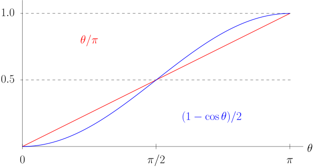
The relaxed contribution is \(\omega_{ij}(1-\cos\theta_{ij})/2\) .
The expected rounded contribution is \(\omega_{ij}\theta_{ij}/\pi\) .
Why a planar picture proves the formula
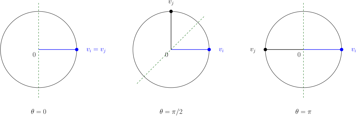
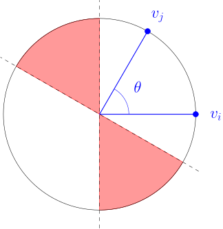
Only the projection of \(r\) onto \(\operatorname{span}\{v_i,v_j\}\) affects the two dot products.
Rotational symmetry makes the projected direction uniform on the circle.
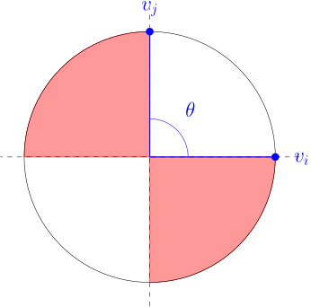
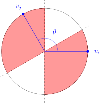
The signs change on the lines perpendicular to \(v_i\) and \(v_j\) .
Equal vectors are never separated; opposite vectors are always separated.
For a noncollinear pair, the span is two-dimensional and the projection is nonzero with probability one. Normalize it without changing signs. Collinear pairs are the endpoint cases theta=0 and theta=pi, handled directly on the last line.
A 60-degree angle
Two sectors of angle \(\theta\) give probability \(2\theta/(2\pi)\) .
For \(\theta=\pi/3\) , the separation probability is \(1/3\) .
A right angle
For \(\theta=\pi/2\) , both the separation probability and the relaxed edge value are \(1/2\) .
A 120-degree angle
For \(\theta=2\pi/3\) , separation probability is \(2/3\) ; relaxed edge value is \(3/4\) .
Two functions to compare
We need a single \(\alpha\) such that
\[\frac{\theta}{\pi}\geq\alpha\frac{1-\cos\theta}{2}
\qquad(0\leq\theta\leq\pi).\]
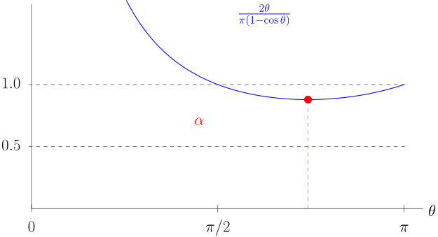
The worst edgewise ratio
\[\alpha=\min_{0<\theta\leq\pi}
\frac{2\theta}{\pi(1-\cos\theta)}\approx0.878567.\]
The minimum occurs near \(\theta=2.331122\) radians.
The derivative vanishes when cos(theta)+theta sin(theta)=1. The generator checks the nonzero solution and numerical value. At theta=0 the ratio is undefined but the edgewise inequality is 0>=0. The source’s closed interval in the ratio definition should therefore be interpreted with this endpoint excluded.
Some edgewise ratios
\(\pi/3\) \(1/3\) \(1/4\) \(4/3\)
\(\pi/2\) \(1/2\) \(1/2\) \(1\)
\(2\pi/3\) \(2/3\) \(3/4\) \(8/9\)
\(\pi\) \(1\) \(1\) \(1\)
Some edges gain; some lose. Every edge retains at least an \(\alpha\) fraction in expectation.
Sum the edgewise guarantee
Let \(W\) be the rounded cut weight, and \(\gamma\) the feasible vector objective.
\[\begin{aligned}
\mathbb E[W]
&=\sum_{i<j}\omega_{ij}\frac{\theta_{ij}}\pi\\
&\geq\alpha\sum_{i<j}\omega_{ij}\frac{1-\cos\theta_{ij}}2\\
&=\alpha\gamma.
\end{aligned}\]
Linearity of expectation does not require different edges to be independent.
The Goemans–Williamson guarantee
For an optimal vector solution,
\[\mathbb E[W]\geq\alpha\gamma^*\geq\alpha\operatorname{OPT},
\qquad\alpha>0.87856.\]
This is an expected approximation guarantee.
A particular random hyperplane can return a worse cut.
Solvers use finite precision
The source’s optimization machinery computes an arbitrarily close approximation.
If a feasible solution has \(\gamma\geq\gamma^*-\eta\) , then
\[\mathbb E[W]\geq\alpha(\gamma^*-\eta)
\geq\alpha\operatorname{OPT}-\alpha\eta.\]
The ideal ratio follows as the solver tolerance tends to zero.
The source initially says the SDP can be solved exactly efficiently, then explicitly qualifies this as approximate optimization. This slide preserves that qualification. Feasibility matters: dot products must come from actual unit vectors, not an arbitrary approximately symmetric array.
Where is the convex optimization problem?
Collect the vectors into the columns of \(V\) and define their Gram matrix
\[M=V^\mathsf{T}V,\qquad M_{ij}=\langle v_i,v_j\rangle.\]
Unit vectors give \(M_{ii}=1\) .
For every \(z\in\mathbb R^n\) ,
\[z^\mathsf{T}Mz=\|Vz\|^2\geq0.\]
Positive semidefinite means a Gram representation
A real symmetric matrix \(M\) is positive semidefinite , written \(M\succeq0\) , if
\[z^\mathsf{T}Mz\geq0\qquad\text{for every }z.\]
Conversely, \(M\succeq0\) admits a factorization \(M=B^\mathsf{T}B\) .
If \(M_{ii}=1\) , the columns of \(B\) are unit vectors ready for rounding.
A spectral square-root factorization handles singular PSD matrices as well. Ordinary strictly positive-pivot Cholesky should not be assumed to work unchanged for every singular PSD input. The notes give O(n^3) for recovering the vectors; use standard dense factorization arithmetic with suitable numerical precision.
The triangle’s Gram matrix
\[M=\begin{pmatrix}
1&-1/2&-1/2\\
-1/2&1&-1/2\\
-1/2&-1/2&1
\end{pmatrix}.\]
The diagonal entries are one. The eigenvalues are \(0,3/2,3/2\) .
This matrix is positive semidefinite, even though it is singular.
It represents the three vectors spaced \(120^\circ\) apart.
Why not make every pair opposite?
An apparent solution would set every off-diagonal entry to \(-1\) :
\[A=\begin{pmatrix}1&-1&-1\\-1&1&-1\\-1&-1&1\end{pmatrix},
\qquad \mathbf1^\mathsf{T}A\mathbf1=-3<0.\]
It is not positive semidefinite, so no unit-vector configuration realizes it.
The PSD constraint enforces consistency among all pairwise dot products.
The semidefinite program
\[\begin{aligned}
\text{maximize}\quad &\frac12\sum_{i<j}\omega_{ij}(1-M_{ij})\\
\text{subject to}\quad &M_{ii}=1\quad(i=1,\ldots,n),\\
&M\succeq0.
\end{aligned}\]
The objective is linear in \(M\) ; the feasible region is convex.
The integrality restriction has become a matrix constraint.
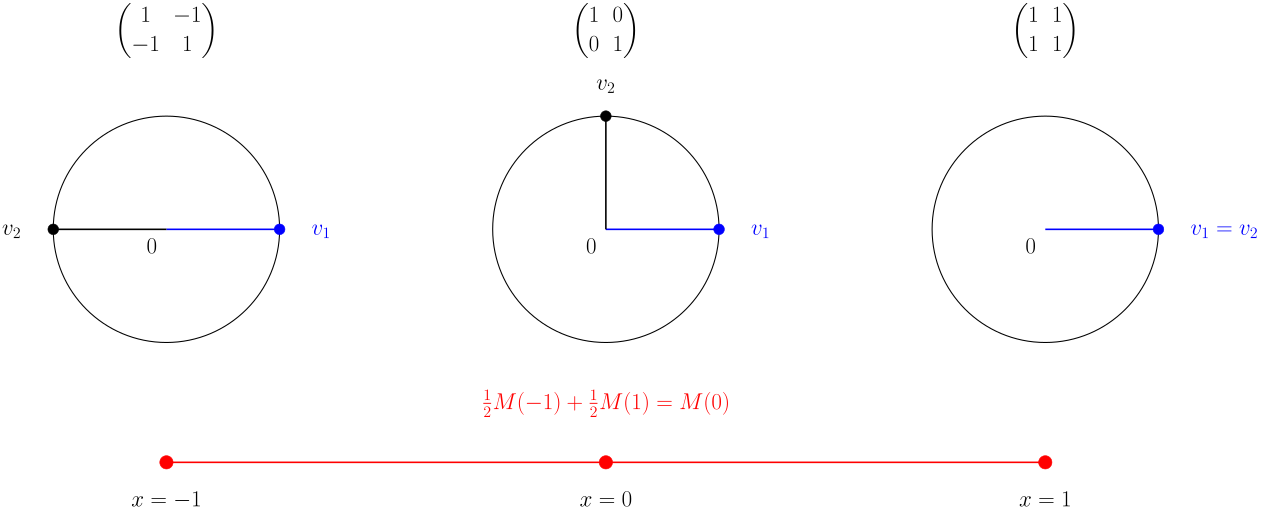
Why the PSD region is convex
Let \(A,B\succeq0\) and \(0\leq t\leq1\) .
For every vector \(z\) ,
\[z^\mathsf{T}(tA+(1-t)B)z
=t\,z^\mathsf{T}Az+(1-t)z^\mathsf{T}Bz\geq0.\]
Thus \(tA+(1-t)B\succeq0\) .
The constraints \(M_{ii}=1\) also survive convex combinations.
Check the max-cut proof
Why is the relaxed optimum an upper bound on MAX CUT?
Why does an angle \(\theta\) give separation probability \(\theta/\pi\) ?
Where do we use nonnegative weights?
Pause about one minute. Every sign solution embeds into vectors; two separating sectors have total angular measure 2theta among 2pi possible normal directions; multiplying and summing the edgewise lower bounds requires nonnegative weights. No independence assumption between edge indicators is used.
Two roles for randomness
Random operation
Contract an edge copy
Choose a hyperplane normal
Object tracked
One fixed optimum
Each edge’s contribution
Main calculation
Conditional survival product
Angle divided by \(\pi\)
Output guarantee
Exact, with high probability
\(\alpha\) approximation in expectation
Contraction preserves a discrete witness.
Rounding converts continuous structure into a discrete solution.
Reading and follow-up
Notes 17 — Min Cut: contraction, amplification, and recursive branching.
Notes 46 — Approximate Max Cut: vector relaxation, angular rounding, and semidefinite programming.
Exercises from the min-cut notes: implement the MST interpretation; reduce FastCut’s space to \(O(n^2)\) .
For the triangle, verify the relaxed optimum \(9/4\) and the rounded value \(2\) .