Dimension Reduction
The Johnson–Lindenstrauss lemma · Mid-length lecture
CS 574 · University of Illinois, Urbana-Champaign · Fall 2026
Storing a point set
Let \(P=\{p_1,\ldots,p_n\}\subseteq\mathbb R^d\).
Coordinates require \(nd\) numbers.
The pairwise distance table requires \(\binom n2\) numbers.
When \(d\) is large, can we store the geometry more economically?
The desired guarantee
Find images \(h(p_i)\in\mathbb R^k\) such that, for every \(i,j\),
\[ (1-\varepsilon)\|p_i-p_j\| \leq\|h(p_i)-h(p_j)\| \leq(1+\varepsilon)\|p_i-p_j\|. \]
Throughout the proof, \(n\geq2\) and \(0<\varepsilon<1/2\).
The random map
Choose independent Gaussian vectors \(u_1,\ldots,u_k\in\mathbb R^d\).
\[h(p)=\frac1{\sqrt k} \bigl(\langle u_1,p\rangle,\ldots,\langle u_k,p\rangle\bigr).\]
Every coordinate of every \(u_i\) is an independent \(N(0,1)\) variable. Use the same map for all points.
Matrix form
\[A=\frac1{\sqrt k} \begin{pmatrix}u_1^\top\\u_2^\top\\\vdots\\u_k^\top\end{pmatrix} \in\mathbb R^{k\times d},\qquad h(p)=Ap.\]
The map is linear. This will let us study differences of points.
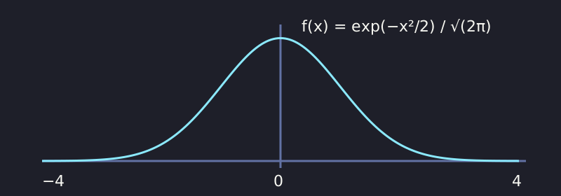
The standard normal density
\[f(x)=\frac1{\sqrt{2\pi}}e^{-x^2/2},\qquad X\sim N(0,1).\]
Two independent normal variables
For independent \(X,Y\sim N(0,1)\), the joint density is
\[g(x,y)=f(x)f(y)=\frac1{2\pi}e^{-(x^2+y^2)/2}.\]
This density depends only on the distance from the origin.
Normalization: square the integral
Let \(I=\int_{-\infty}^{\infty}f(x)\,dx\). Then
\[I^2=\int_{\mathbb R^2} f(x)f(y)\,dx\,dy =\frac1{2\pi}\int_{\mathbb R^2}e^{-(x^2+y^2)/2}\,dx\,dy.\]
The two-dimensional integral has radial symmetry.
Normalization: evaluate
\[\begin{aligned} I^2&=\frac1{2\pi}\int_0^\infty\int_0^{2\pi} e^{-r^2/2}r\,d\theta\,dr\\ &=\int_0^\infty re^{-r^2/2}\,dr =\bigl[-e^{-r^2/2}\bigr]_0^\infty=1. \end{aligned}\]
Since \(I>0\), we have \(I=1\): \(f\) is a probability density.
Variance one
\[x^2e^{-x^2/2}=\bigl(-xe^{-x^2/2}\bigr)'+e^{-x^2/2}.\]
\[\mathbb E[X^2]=\frac1{\sqrt{2\pi}} \bigl[-xe^{-x^2/2}\bigr]_{-\infty}^{\infty} +\int_{-\infty}^{\infty}f(x)\,dx=1.\]
The boundary term vanishes. Hence \(\operatorname{Var}(X)=1\).
A Gaussian vector in \(d\) dimensions
Take independent \(X_1,\ldots,X_d\sim N(0,1)\) and set \(u=(X_1,\ldots,X_d)\).
\[g_d(x)=\prod_{j=1}^d f(x_j) =(2\pi)^{-d/2}\exp\left(-\frac12\sum_{j=1}^d x_j^2\right).\]
Its density integrates to one by the product structure.
Rotational invariance
\[g_d(x)=(2\pi)^{-d/2}e^{-\|x\|^2/2}.\]
For an orthogonal matrix \(R\), \(\|Rx\|=\|x\|\) and \(|\det R|=1\).
Rotation preserves both density and volume, hence probability. The vectors \(Ru\) and \(u\) have the same distribution.
Projection onto a unit direction
Fix \(v\in\mathbb R^d\) with \(\|v\|=1\). Choose a rotation \(R\) with \(Rv=e_1\).
\[\langle v,u\rangle=\langle Rv,Ru\rangle =\langle e_1,Ru\rangle\sim N(0,1).\]
The first coordinate of \(Ru\) has the same distribution as \(X_1\).
One fixed unit vector
Fix \(v\) independently of the sampled matrix, with \(\|v\|=1\).
Set \(X_i=\langle u_i,v\rangle\). Then \[Av=\frac1{\sqrt k}(X_1,\ldots,X_k),\qquad X_i\sim N(0,1).\]
The \(X_i\) are independent because the rows \(u_i\) are independent.
Squared length
\[Y=\sum_{i=1}^k X_i^2,\qquad Z=\frac Yk=\|Av\|^2.\]
\(Y\) has the chi-square distribution with \(k\) degrees of freedom.
The question is now one-dimensional: how concentrated is \(Z\) around \(1\)?
Exponential Markov inequality
For \(0<t<1/2\),
\[\begin{aligned} \Pr[Z\geq1+\varepsilon] &=\Pr[e^{tkZ}\geq e^{tk(1+\varepsilon)}]\\ &\leq e^{-tk(1+\varepsilon)}\mathbb E[e^{tkZ}]. \end{aligned}\]
We need the exponential moment of a squared normal variable.
Independence factors the moment
\[\mathbb E[e^{tkZ}] =\mathbb E\left[\prod_{i=1}^k e^{tX_i^2}\right] =\prod_{i=1}^k\mathbb E[e^{tX_i^2}].\]
All factors are identical. It suffices to compute one integral.
Exponential moment of \(X^2\)
For \(X\sim N(0,1)\) and \(t<1/2\),
\[\mathbb E[e^{tX^2}] =\frac1{\sqrt{2\pi}}\int_{-\infty}^{\infty} e^{-(1-2t)x^2/2}\,dx.\]
Substitute \(y=\sqrt{1-2t}\,x\).
Rescale to a normal density
\[\begin{aligned} \mathbb E[e^{tX^2}] &=\frac1{\sqrt{1-2t}}\, \frac1{\sqrt{2\pi}}\int_{-\infty}^{\infty}e^{-y^2/2}\,dy\\ &=(1-2t)^{-1/2}. \end{aligned}\]
The remaining integral is one by normalization.
Choose the exponential parameter
Set \(t=\varepsilon/4\). Then
\[\Pr[Z\geq1+\varepsilon] \leq\left[ \frac{e^{-(\varepsilon/4)(1+\varepsilon)}}{\sqrt{1-\varepsilon/2}} \right]^k.\]
We next bound the positive contribution of the denominator.
Upper-tail conclusion
\[\boxed{\Pr[Z\geq1+\varepsilon]\leq e^{-k\varepsilon^2/16}.}\]
If \(k\geq16\varepsilon^{-2}\ln(2/\delta)\), the bound is at most \(\delta/2\).
This controls expansion. We still need to control contraction.
Two-sided chi-square tails
For \(Z=k^{-1}\sum_i X_i^2\) and any \(x>0\),
\[\Pr\left[Z\leq1-2\sqrt{x/k}\right]\leq e^{-x},\] \[\Pr\left[Z\geq1+2\sqrt{x/k}+2x/k\right]\leq e^{-x}.\]
Laurent–Massart, Lemma 1 (Laurent & Massart, 2000). Stated without proof, as in the notes.
The dimension bound for concentration
Take \(k\geq8\varepsilon^{-2}\ln(2/\delta)=8\varepsilon^{-2}x\).
\[2\sqrt{x/k}+2x/k \leq\frac\varepsilon{\sqrt2}+\frac{\varepsilon^2}4 \leq\varepsilon\left(\frac1{\sqrt2}+\frac14\right) <\varepsilon.\]
The estimate holds for \(\varepsilon\leq1\); our standing range is smaller.
Concentration corollary
If \(0<\delta<1\), \(0<\varepsilon<1/2\), and
\[k\geq\left\lceil8\varepsilon^{-2}\ln(2/\delta)\right\rceil,\]
then \[\boxed{\Pr[1-\varepsilon\leq Z\leq1+\varepsilon]\geq1-\delta.}\]
This is the two-sided estimate used in the JL proof.
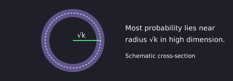
Gaussian mass in a thin shell
For \(X=(X_1,\ldots,X_k)\),
\[Z=\frac{\|X\|^2}{k}\approx1 \quad\Longrightarrow\quad \|X\|\approx\sqrt k.\]
Squared length to length
For \(0<\varepsilon<1\),
\[1-\varepsilon\leq\sqrt{1-\varepsilon}, \qquad\sqrt{1+\varepsilon}\leq1+\varepsilon.\]
Thus \(1-\varepsilon\leq\|Av\|^2\leq1+\varepsilon\) implies \[1-\varepsilon\leq\|Av\|\leq1+\varepsilon.\]
Failure budget for one direction
Set \(\delta=1/n^2\).
For \(n\geq2\), \[8\varepsilon^{-2}\ln(2n^2) \leq24\varepsilon^{-2}\ln n.\]
Our choice \(k=\lceil24\varepsilon^{-2}\ln n\rceil\) is sufficient.
Linearity preserves differences
\[Ap-Aq=A(p-q)=\|p-q\|Av_{pq}.\]
Therefore \[\frac{\|Ap-Aq\|}{\|p-q\|}=\|Av_{pq}\|.\]
Here \(v_{pq}=(p-q)/\|p-q\|\) for distinct \(p,q\). Distance distortion equals length distortion in this unit direction.
Union bound over all pairs
\[\Pr\left[\bigcup_{\{p,q\}\subseteq P}B_{pq}\right] \leq\sum_{\{p,q\}\subseteq P}\Pr[B_{pq}] \leq\binom n2\frac1{n^2} =\frac{n-1}{2n}<\frac12.\]
Here \(B_{pq}\) is the failure event for pair \(p,q\), with probability at most \(1/n^2\). Independence between pair events is unnecessary.
The Johnson–Lindenstrauss lemma
Given \(n\) points in \(\mathbb R^d\) and \(0<\varepsilon<1/2\), there is a map into
\[\mathbb R^k,\qquad k=O(\varepsilon^{-2}\log n),\]
that preserves every pairwise distance within a factor \(1\pm\varepsilon\).
The Gaussian construction succeeds with probability at least \(1/2\).
Shift and rescale a standard normal
Let \(X\sim N(0,1)\) and \(Y=\sigma X+\mu\), with \(\sigma>0\).
\[f_{\mu,\sigma}(y)=\frac1{\sqrt{2\pi}\sigma} \exp\left(-\frac{(y-\mu)^2}{2\sigma^2}\right).\]
We write \(Y\sim N(\mu,\sigma^2)\).
A weighted sum of two normals
Let \(X,Y\) be independent \(N(0,1)\) variables and \(\alpha,\beta>0\).
\[\sigma=\sqrt{\alpha^2+\beta^2},\qquad v=\frac{(\alpha,\beta)}{\sigma}.\]
Since \(\|v\|=1\), \(\langle v,(X,Y)\rangle\sim N(0,1)\).
Thus \(\alpha X+\beta Y\sim N(0,\alpha^2+\beta^2)\).
Sum of independent normal variables
If \(X\sim N(\mu_1,\sigma_1^2)\) and \(Y\sim N(\mu_2,\sigma_2^2)\) are independent,
\[\boxed{X+Y\sim N(\mu_1+\mu_2,\sigma_1^2+\sigma_2^2).}\]
Write \(X=\sigma_1\widehat X+\mu_1\) and \(Y=\sigma_2\widehat Y+\mu_2\), then use the weighted-sum result and shift by \(\mu_1+\mu_2\).
References
CS 574 · Dimension reduction · Notes 26