Dimension Reduction
The Johnson–Lindenstrauss lemma · Full lecture
CS 574 · University of Illinois, Urbana-Champaign · Fall 2026
The route to dimension reduction
Compress a finite point set while approximately preserving every pairwise distance.
| Topic | Minutes |
|---|---|
| Problem and random map | 10 |
| Normal distribution and rotational symmetry | 20 |
| Concentration of squared length | 25 |
| Pairwise distances and the JL lemma | 15 |
| Additional Gaussian facts | 5 |
Storing a point set
Let \(P=\{p_1,\ldots,p_n\}\subseteq\mathbb R^d\).
Coordinates require \(nd\) numbers.
The pairwise distance table requires \(\binom n2\) numbers.
When \(d\) is large, can we store the geometry more economically?
The desired guarantee
Find images \(h(p_i)\in\mathbb R^k\) such that, for every \(i,j\),
\[ (1-\varepsilon)\|p_i-p_j\| \leq\|h(p_i)-h(p_j)\| \leq(1+\varepsilon)\|p_i-p_j\|. \]
Throughout the proof, \(n\geq2\) and \(0<\varepsilon<1/2\).
Target dimension
\[k=\left\lceil24\varepsilon^{-2}\ln n\right\rceil.\]
The image coordinates use \(nk\) numbers.
The bound depends on the number of points and the allowed distortion. It is independent of the original dimension \(d\).
The random map
Choose independent Gaussian vectors \(u_1,\ldots,u_k\in\mathbb R^d\).
\[h(p)=\frac1{\sqrt k} \bigl(\langle u_1,p\rangle,\ldots,\langle u_k,p\rangle\bigr).\]
Every coordinate of every \(u_i\) is an independent \(N(0,1)\) variable. Use the same map for all points.
Matrix form
\[A=\frac1{\sqrt k} \begin{pmatrix}u_1^\top\\u_2^\top\\\vdots\\u_k^\top\end{pmatrix} \in\mathbb R^{k\times d},\qquad h(p)=Ap.\]
The map is linear. This will let us study differences of points.
Why Gaussian coordinates?
A Gaussian vector has the same distribution after a rotation.
Its projection onto any fixed unit direction is \(N(0,1)\).
We first establish these facts, then use them to analyze \(\|Av\|\).
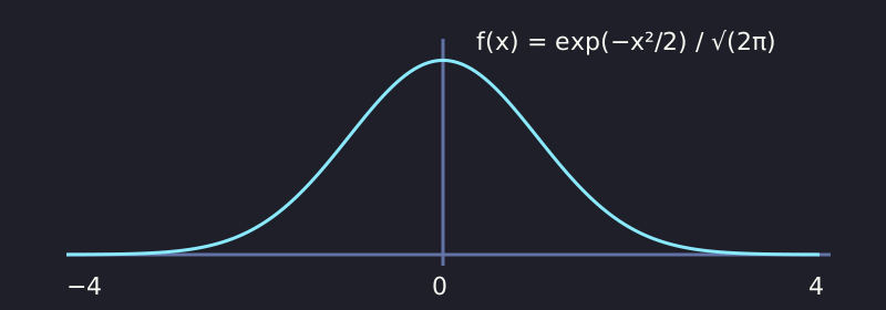
The standard normal density
\[f(x)=\frac1{\sqrt{2\pi}}e^{-x^2/2},\qquad X\sim N(0,1).\]
Two independent normal variables
For independent \(X,Y\sim N(0,1)\), the joint density is
\[g(x,y)=f(x)f(y)=\frac1{2\pi}e^{-(x^2+y^2)/2}.\]
This density depends only on the distance from the origin.
Equal density on circles
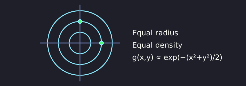
\[x^2+y^2=(x')^2+(y')^2\quad\Longrightarrow\quad g(x,y)=g(x',y').\]
Normalization: square the integral
Let \(I=\int_{-\infty}^{\infty}f(x)\,dx\). Then
\[I^2=\int_{\mathbb R^2} f(x)f(y)\,dx\,dy =\frac1{2\pi}\int_{\mathbb R^2}e^{-(x^2+y^2)/2}\,dx\,dy.\]
The two-dimensional integral has radial symmetry.
Polar coordinates
\[x=r\cos\theta,\qquad y=r\sin\theta.\]
\[\left|\det \begin{pmatrix}\cos\theta&-r\sin\theta\\ \sin\theta&r\cos\theta\end{pmatrix}\right|=r.\]
Thus \(dx\,dy=r\,dr\,d\theta\).
Normalization: evaluate
\[\begin{aligned} I^2&=\frac1{2\pi}\int_0^\infty\int_0^{2\pi} e^{-r^2/2}r\,d\theta\,dr\\ &=\int_0^\infty re^{-r^2/2}\,dr =\bigl[-e^{-r^2/2}\bigr]_0^\infty=1. \end{aligned}\]
Since \(I>0\), we have \(I=1\): \(f\) is a probability density.
Mean zero
\[\mathbb E[X]=\int_{-\infty}^{\infty}x f(x)\,dx=0.\]
The density is even, so \(x f(x)\) is odd. The contributions on the two sides of zero cancel.
Variance: reduce to an integral
\[\operatorname{Var}(X)=\mathbb E[X^2]-(\mathbb E[X])^2 =\frac1{\sqrt{2\pi}}\int_{-\infty}^{\infty}x^2e^{-x^2/2}\,dx.\]
Use the derivative of \(-xe^{-x^2/2}\).
Variance one
\[x^2e^{-x^2/2}=\bigl(-xe^{-x^2/2}\bigr)'+e^{-x^2/2}.\]
\[\mathbb E[X^2]=\frac1{\sqrt{2\pi}} \bigl[-xe^{-x^2/2}\bigr]_{-\infty}^{\infty} +\int_{-\infty}^{\infty}f(x)\,dx=1.\]
The boundary term vanishes. Hence \(\operatorname{Var}(X)=1\).
A Gaussian vector in \(d\) dimensions
Take independent \(X_1,\ldots,X_d\sim N(0,1)\) and set \(u=(X_1,\ldots,X_d)\).
\[g_d(x)=\prod_{j=1}^d f(x_j) =(2\pi)^{-d/2}\exp\left(-\frac12\sum_{j=1}^d x_j^2\right).\]
Its density integrates to one by the product structure.
Rotational invariance
\[g_d(x)=(2\pi)^{-d/2}e^{-\|x\|^2/2}.\]
For an orthogonal matrix \(R\), \(\|Rx\|=\|x\|\) and \(|\det R|=1\).
Rotation preserves both density and volume, hence probability. The vectors \(Ru\) and \(u\) have the same distribution.
Projection onto a unit direction
Fix \(v\in\mathbb R^d\) with \(\|v\|=1\). Choose a rotation \(R\) with \(Rv=e_1\).
\[\langle v,u\rangle=\langle Rv,Ru\rangle =\langle e_1,Ru\rangle\sim N(0,1).\]
The first coordinate of \(Ru\) has the same distribution as \(X_1\).
Gaussian facts needed for JL
- Independent standard normals form a Gaussian vector.
- Its distribution is invariant under rotations.
- Projection onto a fixed unit vector is standard normal.
These facts remove the original dimension from the length analysis.
One fixed unit vector
Fix \(v\) independently of the sampled matrix, with \(\|v\|=1\).
Set \(X_i=\langle u_i,v\rangle\). Then \[Av=\frac1{\sqrt k}(X_1,\ldots,X_k),\qquad X_i\sim N(0,1).\]
The \(X_i\) are independent because the rows \(u_i\) are independent.
Squared length
\[Y=\sum_{i=1}^k X_i^2,\qquad Z=\frac Yk=\|Av\|^2.\]
\(Y\) has the chi-square distribution with \(k\) degrees of freedom.
The question is now one-dimensional: how concentrated is \(Z\) around \(1\)?
The scale factor
\[\mathbb E[Y]=\sum_{i=1}^k\mathbb E[X_i^2]=k, \qquad \mathbb E[Z]=1.\]
This explains the factor \(1/\sqrt k\) in the map. Expectation alone does not give the probability bound we need.
An upper-tail estimate
For \(0<\varepsilon<1/2\), we will prove
\[\Pr[Z\geq1+\varepsilon]\leq e^{-k\varepsilon^2/16}.\]
This is the Chernoff method: exponentiate, apply Markov’s inequality, and use independence.
Exponential Markov inequality
For \(0<t<1/2\),
\[\begin{aligned} \Pr[Z\geq1+\varepsilon] &=\Pr[e^{tkZ}\geq e^{tk(1+\varepsilon)}]\\ &\leq e^{-tk(1+\varepsilon)}\mathbb E[e^{tkZ}]. \end{aligned}\]
We need the exponential moment of a squared normal variable.
Independence factors the moment
\[\mathbb E[e^{tkZ}] =\mathbb E\left[\prod_{i=1}^k e^{tX_i^2}\right] =\prod_{i=1}^k\mathbb E[e^{tX_i^2}].\]
All factors are identical. It suffices to compute one integral.
Exponential moment of \(X^2\)
For \(X\sim N(0,1)\) and \(t<1/2\),
\[\mathbb E[e^{tX^2}] =\frac1{\sqrt{2\pi}}\int_{-\infty}^{\infty} e^{-(1-2t)x^2/2}\,dx.\]
Substitute \(y=\sqrt{1-2t}\,x\).
Rescale to a normal density
\[\begin{aligned} \mathbb E[e^{tX^2}] &=\frac1{\sqrt{1-2t}}\, \frac1{\sqrt{2\pi}}\int_{-\infty}^{\infty}e^{-y^2/2}\,dy\\ &=(1-2t)^{-1/2}. \end{aligned}\]
The remaining integral is one by normalization.
Choose the exponential parameter
Set \(t=\varepsilon/4\). Then
\[\Pr[Z\geq1+\varepsilon] \leq\left[ \frac{e^{-(\varepsilon/4)(1+\varepsilon)}}{\sqrt{1-\varepsilon/2}} \right]^k.\]
We next bound the positive contribution of the denominator.
A geometric-series bound
Put \(q=\varepsilon/2\) and \(S=\sum_{j\geq1}q^j\). Then
\[\frac1{1-q}=1+S\leq(1+S/2)^2\leq e^S.\]
Therefore \((1-q)^{-1/2}\leq e^{S/2}\).
This is the geometric-series estimate used in the notes.
Cancellation in the exponent
\[\begin{aligned} \frac12\sum_{j\geq1}(\varepsilon/2)^j -\frac\varepsilon4(1+\varepsilon) &=\frac\varepsilon4+\frac{\varepsilon^2}8 -\frac\varepsilon4-\frac{\varepsilon^2}4 +\frac12\sum_{j\geq3}(\varepsilon/2)^j\\ &=-\frac{\varepsilon^2}8 +\frac12\sum_{j\geq3}(\varepsilon/2)^j. \end{aligned}\]
The linear terms cancel, leaving a negative quadratic term.
Bound the remainder
Since \(0<\varepsilon<1/2\),
\[\frac12\sum_{j\geq3}(\varepsilon/2)^j =\frac{(\varepsilon/2)^3}{2(1-\varepsilon/2)} \leq(\varepsilon/2)^3\leq\frac{\varepsilon^2}{16}.\]
The exponent is at most \(-\varepsilon^2/16\) per factor.
Upper-tail conclusion
\[\boxed{\Pr[Z\geq1+\varepsilon]\leq e^{-k\varepsilon^2/16}.}\]
If \(k\geq16\varepsilon^{-2}\ln(2/\delta)\), the bound is at most \(\delta/2\).
This controls expansion. We still need to control contraction.
Two-sided chi-square tails
For \(Z=k^{-1}\sum_i X_i^2\) and any \(x>0\),
\[\Pr\left[Z\leq1-2\sqrt{x/k}\right]\leq e^{-x},\] \[\Pr\left[Z\geq1+2\sqrt{x/k}+2x/k\right]\leq e^{-x}.\]
Laurent–Massart, Lemma 1 (Laurent & Massart, 2000). Stated without proof, as in the notes.
Allocate the failure probability
Choose \(x=\ln(2/\delta)\), so \(e^{-x}=\delta/2\).
It suffices that \[2\sqrt{x/k}\leq\varepsilon, \qquad 2\sqrt{x/k}+2x/k\leq\varepsilon.\]
Then the two tails together have probability at most \(\delta\).
The dimension bound for concentration
Take \(k\geq8\varepsilon^{-2}\ln(2/\delta)=8\varepsilon^{-2}x\).
\[2\sqrt{x/k}+2x/k \leq\frac\varepsilon{\sqrt2}+\frac{\varepsilon^2}4 \leq\varepsilon\left(\frac1{\sqrt2}+\frac14\right) <\varepsilon.\]
The estimate holds for \(\varepsilon\leq1\); our standing range is smaller.
Concentration corollary
If \(0<\delta<1\), \(0<\varepsilon<1/2\), and
\[k\geq\left\lceil8\varepsilon^{-2}\ln(2/\delta)\right\rceil,\]
then \[\boxed{\Pr[1-\varepsilon\leq Z\leq1+\varepsilon]\geq1-\delta.}\]
This is the two-sided estimate used in the JL proof.
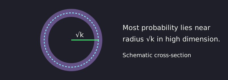
Gaussian mass in a thin shell
For \(X=(X_1,\ldots,X_k)\),
\[Z=\frac{\|X\|^2}{k}\approx1 \quad\Longrightarrow\quad \|X\|\approx\sqrt k.\]
Squared length to length
For \(0<\varepsilon<1\),
\[1-\varepsilon\leq\sqrt{1-\varepsilon}, \qquad\sqrt{1+\varepsilon}\leq1+\varepsilon.\]
Thus \(1-\varepsilon\leq\|Av\|^2\leq1+\varepsilon\) implies \[1-\varepsilon\leq\|Av\|\leq1+\varepsilon.\]
Failure budget for one direction
Set \(\delta=1/n^2\).
For \(n\geq2\), \[8\varepsilon^{-2}\ln(2n^2) \leq24\varepsilon^{-2}\ln n.\]
Our choice \(k=\lceil24\varepsilon^{-2}\ln n\rceil\) is sufficient.
One-vector preservation lemma
For any fixed unit vector \(v\in\mathbb R^d\),
\[\boxed{\Pr[1-\varepsilon\leq\|Av\|\leq1+\varepsilon] \geq1-\frac1{n^2}.}\]
The probability is over the random matrix \(A\). The vector \(v\) is fixed before drawing \(A\).
Differences of points
For distinct \(p,q\in P\), define
\[v_{pq}=\frac{p-q}{\|p-q\|}.\]
This is a fixed unit vector. Apply the one-vector lemma to it.
Linearity preserves differences
\[Ap-Aq=A(p-q)=\|p-q\|Av_{pq}.\]
Therefore \[\frac{\|Ap-Aq\|}{\|p-q\|}=\|Av_{pq}\|.\]
Distance distortion is exactly length distortion in the difference direction.
Guarantee for one pair
With probability at least \(1-1/n^2\),
\[ (1-\varepsilon)\|p-q\| \leq\|Ap-Aq\| \leq(1+\varepsilon)\|p-q\|.\]
For \(p=q\) the inequality holds automatically.
The finite collection of directions
There are \(\binom n2\) unordered pairs of distinct points.
For each pair, let \(B_{pq}\) be the event that its distance is not preserved. \[\Pr[B_{pq}]\leq\frac1{n^2}.\]
The events can be dependent: every pair uses the same matrix.
Union bound over all pairs
\[\Pr\left[\bigcup_{\{p,q\}\subseteq P}B_{pq}\right] \leq\sum_{\{p,q\}\subseteq P}\Pr[B_{pq}] \leq\binom n2\frac1{n^2} =\frac{n-1}{2n}<\frac12.\]
Independence between pair events is unnecessary.
Simultaneous preservation
With probability at least \(1/2\), all pairs \(p,q\in P\) satisfy
\[ (1-\varepsilon)\|p-q\| \leq\|Ap-Aq\| \leq(1+\varepsilon)\|p-q\|.\]
One successful matrix embeds the entire point set.
The Johnson–Lindenstrauss lemma
Given \(n\) points in \(\mathbb R^d\) and \(0<\varepsilon<1/2\), there is a map into
\[\mathbb R^k,\qquad k=O(\varepsilon^{-2}\log n),\]
that preserves every pairwise distance within a factor \(1\pm\varepsilon\).
The Gaussian construction succeeds with probability at least \(1/2\).
Construction and proof together
- Set \(k=\lceil24\varepsilon^{-2}\ln n\rceil\).
- Sample independent \(u_i\sim N(0,I_d)\); use rows \(u_i^\top/\sqrt k\).
- Map every point by \(h(p)=Ap\).
- Chi-square concentration controls each fixed difference direction.
- A union bound controls all \(\binom n2\) pairs.
What the guarantee covers
The finite input set \(P\) is fixed before sampling \(A\).
The guarantee concerns every pair in that set.
The proof uses finitely many directions \(v_{pq}\); it does not assert simultaneous preservation of all vectors in \(\mathbb R^d\).
Space after reduction
Original point coordinates: \(nd\) numbers.
Image coordinates: \(nk=O(n\varepsilon^{-2}\log n)\) numbers.
The reduction is useful when the target dimension is much smaller than \(d\). This count is for the point representation, as in the notes.
Proof dependencies
Gaussian symmetry \(\Longrightarrow\) normal projections.
Normal projections \(\Longrightarrow\) chi-square squared length.
Concentration \(\Longrightarrow\) one direction is preserved.
Linearity and a union bound \(\Longrightarrow\) all pairwise distances are preserved.
Additional Gaussian facts
The remaining facts are supplementary material from the notes.
They are not needed for the dimension-reduction proof.
We examine shifts, rescaling, and sums of independent normals.
Shift and rescale a standard normal
Let \(X\sim N(0,1)\) and \(Y=\sigma X+\mu\), with \(\sigma>0\).
\[f_{\mu,\sigma}(y)=\frac1{\sqrt{2\pi}\sigma} \exp\left(-\frac{(y-\mu)^2}{2\sigma^2}\right).\]
We write \(Y\sim N(\mu,\sigma^2)\).
Derive the transformed density
\[\begin{aligned} \Pr[Y\leq a] &=\Pr[X\leq(a-\mu)/\sigma]\\ &=\int_{-\infty}^{(a-\mu)/\sigma}f(x)\,dx\\ &=\int_{-\infty}^a\frac1\sigma f\left(\frac{y-\mu}{\sigma}\right)\,dy. \end{aligned}\]
The substitution is \(y=\sigma x+\mu\).
Mean and variance after scaling
\[\mathbb E[\sigma X+\mu]=\sigma\mathbb E[X]+\mu=\mu,\]
\[\operatorname{Var}(\sigma X+\mu)=\sigma^2\operatorname{Var}(X)=\sigma^2.\]
The second parameter in \(N(\mu,\sigma^2)\) is the variance.
A weighted sum of two normals
Let \(X,Y\) be independent \(N(0,1)\) variables and \(\alpha,\beta>0\).
\[\sigma=\sqrt{\alpha^2+\beta^2},\qquad v=\frac{(\alpha,\beta)}{\sigma}.\]
Since \(\|v\|=1\), \(\langle v,(X,Y)\rangle\sim N(0,1)\).
Thus \(\alpha X+\beta Y\sim N(0,\alpha^2+\beta^2)\).
The halfspace interpretation
\[\{(x,y):\alpha x+\beta y\leq z\} =\{(x,y):\langle v,(x,y)\rangle\leq z/\sigma\}.\]
Rotate \(v\) to the first coordinate direction. Rotational invariance gives the probability \(\Pr[X\leq z/\sigma]\).
The boundary has signed offset \(z/\sigma\) and distance \(|z|/\sigma\) from the origin.
Sum of independent normal variables
If \(X\sim N(\mu_1,\sigma_1^2)\) and \(Y\sim N(\mu_2,\sigma_2^2)\) are independent,
\[\boxed{X+Y\sim N(\mu_1+\mu_2,\sigma_1^2+\sigma_2^2).}\]
Write \(X=\sigma_1\widehat X+\mu_1\) and \(Y=\sigma_2\widehat Y+\mu_2\), then use the weighted-sum result and shift by \(\mu_1+\mu_2\).
Bibliographical notes
The JL lemma is due to Johnson and Lindenstrauss (Johnson & Lindenstrauss, 1984).
The notes follow class notes of Anupam Gupta, in turn following Indyk and Motwani (Indyk & Motwani, 1998).
The two-sided chi-square estimate is from Laurent and Massart (Laurent & Massart, 2000).
References
CS 574 · Dimension reduction · Notes 26