---
output-file: index.html
title: "Frequency Estimation over a Stream"
subtitle: "Notes 28 · Full lecture · 75 minutes"
author: "Sariel Har-Peled"
institute: "CS 574 · University of Illinois, Urbana-Champaign · Fall 2026"
---

## Three steps to a streaming estimate

::: {.card-cyan}
### Build → analyze → amplify
An unbiased random variable is the starting point.
Control its variance, average independent copies, then take a median.
:::

::: {.card-green}
| Part | Minutes |
|:---|---:|
| Model and frequency moments | 5 |
| Averaging and median amplification | 15 |
| A reservoir estimator for $F_k$ | 25 |
| A smaller sketch for $F_2$ | 25 |
| Guarantees and discussion | 5 |
:::

::: {.notes}
Source: frequency_est.tex, Chapter 28, with the verified repairs recorded
in ../CORRECTIONS.txt. Time allocations include questions and board work.
The full deck deliberately separates steps in the proofs.
:::

## The stream and its frequency vector

::: {.card-purple}
$$
\sigma=(s_1,\ldots,s_m),\qquad s_t\in[n]=\{1,\ldots,n\}.
$$
$$
f_i=|\{t:s_t=i\}|,\qquad \sum_{i=1}^n f_i=m.
$$
$m$ counts positions; $n$ is the universe size.
:::

::: {.card-cyan}
One pass through an insertion-only stream; memory much smaller than a full frequency table.
:::

## Frequency moments

::: {.card-green}
$$
F_k=\sum_{i=1}^n f_i^k.
$$
$$
F_0=|\{i:f_i>0\}|,\quad F_1=m,\quad
F_2=\sum_i f_i^2,\quad F_\infty=\max_i f_i.
$$
For $F_0$, use $0^0=0$ and $a^0=1$ for $a>0$.
:::

::: {.card-orange}
Today: $F_k$ for fixed integer $k\geq1$, then a better bound for $F_2$.
:::

## What does a successful estimate mean?

::: {.card-purple}
For $0<\varepsilon,\delta<1$, return $\widehat F_k$ satisfying
$$
\Pr\bigl[|\widehat F_k-F_k|>\varepsilon F_k\bigr]\leq\delta.
$$
The probability is over the algorithm's randomness, for any fixed stream.
:::

::: {.card-cyan}
Words hold an item identifier or a stream counter.
For fixed $k$, a constant number of words also holds the needed powers.
An empty stream is handled separately: return $0$.
:::

## Unbiased is not yet accurate

::: {.card-orange}
### The coin example
$$
X\sim\operatorname{Bernoulli}(p),\qquad \mathbb E X=p,
\qquad \operatorname{Var}(X)=p(1-p).
$$
One flip returns $0$ or $1$, even when the target is a small positive $p$.
:::

::: {.card-green}
We need a bound on deviation from the mean, not just the correct mean.
:::

## The abstract estimation problem

::: {.card-cyan}
$$
\mathbb E X=\mu>0,\qquad
\operatorname{Var}(X)=\nu<\infty.
$$
Construct $Z$ with
$$
\Pr[(1-\varepsilon)\mu\leq Z\leq(1+\varepsilon)\mu]\geq1-\delta.
$$
:::

::: {.card-purple}
The useful quantity is the relative variance $\nu/\mu^2$.
:::

## Chebyshev sets the variance target

::: {.card-green}
For any $a>0$,
$$
\Pr[|W-\mathbb E W|\geq a]
\leq\frac{\operatorname{Var}(W)}{a^2}.
$$
If $\mathbb E W=\mu$ and $\operatorname{Var}(W)\leq\varepsilon^2\mu^2/4$, then
$$
\Pr[|W-\mu|\geq\varepsilon\mu]\leq\frac14.
$$
:::

::: {.notes}
This form also covers variance zero; no division by a standard deviation.
:::

## Average independent samples

::: {.card-purple}
$$
X_1,\ldots,X_\alpha\text{ independent copies of }X,
\qquad A=\frac1\alpha\sum_{j=1}^\alpha X_j.
$$
$$
\mathbb E A=\frac1\alpha\sum_j\mathbb E X_j=\mu.
$$
:::

::: {.card-cyan}
Averaging preserves the target mean.
:::

## Independence reduces variance

::: {.card-green}
$$
\begin{aligned}
\operatorname{Var}(A)
&=\frac1{\alpha^2}\operatorname{Var}\left(\sum_jX_j\right)\\
&=\frac1{\alpha^2}\sum_j\operatorname{Var}(X_j)
=\frac\nu\alpha.
\end{aligned}
$$
:::

::: {.card-orange}
Repeatedly using the same random sample would not reduce variance.
:::

## Choose the block size

::: {.card-purple}
$$
\alpha=\max\left\{1,\left\lceil\frac{4\nu}{\varepsilon^2\mu^2}\right\rceil\right\}.
$$
$$
\Pr[|A-\mu|\geq\varepsilon\mu]
\leq\frac\nu{\alpha\varepsilon^2\mu^2}\leq\frac14.
$$
:::

::: {.card-cyan}
If $\nu=0$, one sample is already exact. In an algorithm, a known upper bound on $\nu/\mu^2$ suffices.
:::

## Why a second layer?

::: {.card-orange}
Chebyshev applied to one average of $M$ samples gives
$$
\Pr[\text{failure}]\leq\frac\nu{M\varepsilon^2\mu^2}.
$$
This route uses $M\geq\nu/(\delta\varepsilon^2\mu^2)$ for failure $\delta$.
:::

::: {.card-green}
The median of independent averages needs only logarithmically many blocks in $1/\delta$.
:::

## Median of averages

::: {.card-purple}
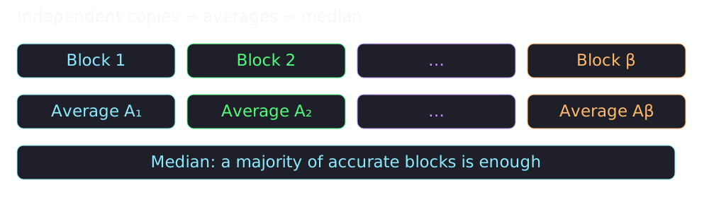
$$
A_i=\frac1\alpha\sum_{j=1}^\alpha X_{i,j},\qquad
Z=\operatorname{median}(A_1,\ldots,A_\beta).
$$
All $\alpha\beta$ samples are independent; take $\beta$ odd.
:::

![](../figs/median.svg){fig-alt="Independent blocks are averaged; their averages feed one median." width=1000}

## A majority inside the interval traps the median

::: {.card-cyan}
Let $I=[(1-\varepsilon)\mu,(1+\varepsilon)\mu]$.
$$
G_i=\mathbf1[A_i\in I],\qquad G=\sum_{i=1}^{\beta}G_i.
$$
$$
\Pr[G_i=1]\geq\frac34,\qquad \mathbb E G\geq\frac{3\beta}{4}.
$$
:::

::: {.card-green}
$$
G>\beta/2\ \Longrightarrow\ Z\in I.
$$
A bad median therefore implies $G<\beta/2$.
:::

## Chernoff bounds the bad majority

::: {.card-purple}
For independent Bernoulli variables and $0<t<1$,
$$
\Pr[G<(1-t)\mathbb E G]\leq e^{-t^2\mathbb E G/2}.
$$
Since $\beta/2\leq(2/3)\mathbb E G$,
$$
\Pr[Z\notin I]\leq e^{-\mathbb E G/18}\leq e^{-\beta/24}.
$$
:::

## A complete amplification theorem

::: {.card-green}
Choose
$$
\alpha=\max\{1,\lceil4\nu/(\varepsilon^2\mu^2)\rceil\},
\qquad \beta=2\lceil12\ln(1/\delta)\rceil+1.
$$
Using $M=\alpha\beta$ independent samples,
$$
\Pr[|Z-\mu|>\varepsilon\mu]\leq\delta.
$$
:::

::: {.card-cyan}
$$
M=O\left(\left(1+\frac\nu{\varepsilon^2\mu^2}\right)
\log\frac2\delta\right).
$$
Compute block averages and select their median in $O(M)$ time.
:::

::: {.notes}
End the estimation segment near minute 20. Ask which part controls accuracy
and which part controls confidence: block size versus number of blocks.
:::

## Return to the stream

::: {.card-purple}
Goal: one constant-size random sketch $X$ with $\mathbb E X=F_k$.
:::

::: {.card-green}
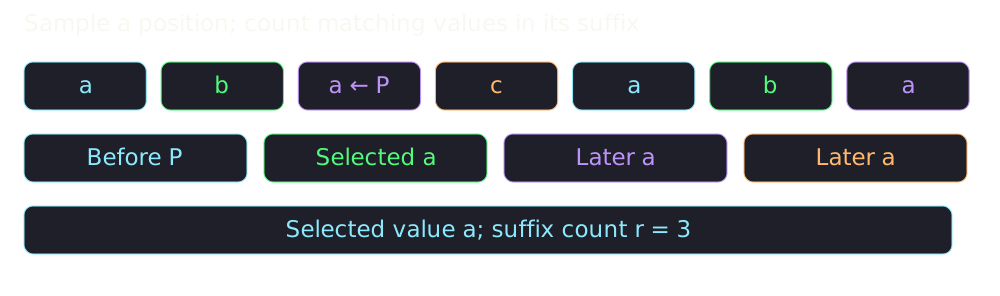
Pick a uniformly random stream position $P\in[m]$.
Store its value and count its occurrences from position $P$ onward.
:::

## A random position, not a random distinct value

::: {.card-cyan}
$$
\Pr[P=t]=1/m,\qquad
\Pr[s_P=i]=f_i/m.
$$
Frequent values are more likely to be selected.
:::

![](../figs/reservoir.svg){fig-alt="A stream with a selected occurrence; only equal values in the suffix contribute to the counter." width=1000}

## Reservoir sampling implements that choice

::: {.card-purple}
At position $t$, replace the representative with $s_t$ with probability $1/t$.
:::

::: {.card-green}
For a fixed position $p\leq m$,
$$
\Pr[P=p]=\frac1p\prod_{t=p+1}^m\left(1-\frac1t\right)
=\frac1p\cdot\frac pm=\frac1m.
$$
The final position is uniform without knowing $m$ in advance.
:::

## Maintain the suffix count

::: {.card-purple}
State: position counter $t$, representative $v$, suffix counter $r$.

On arrival of $s_t$:

1. With probability $1/t$, set $v\gets s_t$ and $r\gets1$.
2. Otherwise, if $s_t=v$, set $r\gets r+1$.
:::

::: {.card-orange}
Replacement resets $r$ even when the new representative has the same value.
:::

## What does the final counter represent?

::: {.card-cyan}
If the final selected position is $P$, then
$$
r=|\{t\geq P:s_t=s_P\}|.
$$
For a value appearing $f_i$ times, the suffix ranks at its occurrences are
$$
f_i,f_i-1,\ldots,1.
$$
:::

## Use a discrete derivative

::: {.card-purple}
$$
\Delta_k(r)=r^k-(r-1)^k,\qquad X=m\Delta_k(r).
$$
:::

::: {.card-green}
$$
\sum_{r=1}^{f_i}\Delta_k(r)=f_i^k-0^k=f_i^k.
$$
The difference is chosen so the expectation telescopes.
:::

## Unbiasedness: sum over all positions

::: {.card-green}
$$
\begin{aligned}
\mathbb E X
&=\frac1m\sum_{i=1}^n\sum_{r=1}^{f_i}m\Delta_k(r)\\
&=\sum_{i=1}^n\sum_{r=1}^{f_i}\bigl(r^k-(r-1)^k\bigr)\\
&=\sum_{i=1}^n f_i^k=F_k.
\end{aligned}
$$
:::

::: {.notes}
Absent values contribute empty sums, so no conditioning on zero-probability
events is necessary. Pause to have the class identify the telescoping sum.
:::

## Check the first moment

::: {.card-cyan}
For $k=1$,
$$
X=m\bigl(r-(r-1)\bigr)=m=F_1.
$$
The estimator is deterministic and exact.
:::

::: {.card-orange}
The interesting variance analysis begins at $k>1$.
:::

## Check the second moment estimator

::: {.card-purple}
For $k=2$,
$$
X=m\bigl(r^2-(r-1)^2\bigr)=m(2r-1).
$$
For a value of frequency $f$,
$$
1+3+\cdots+(2f-1)=f^2.
$$
:::

::: {.notes}
This is the same telescoping proof made concrete. Do not confuse the target
frequency moment F_2 with the probabilistic second moment E[X^2].
:::

## The telescoping idea is more general

::: {.card-green}
Let $g(0)=0$, and set
$$
X_g=m\bigl(g(r)-g(r-1)\bigr).
$$
Then
$$
\mathbb E X_g=\sum_{i=1}^n g(f_i).
$$
:::

::: {.card-orange}
This establishes the mean. A useful approximation still needs a variance bound.
:::

## Bound one increment

::: {.card-cyan}
For $r\geq1$ and $k\geq1$,
$$
0\leq\Delta_k(r)=\int_{r-1}^r kx^{k-1}\,dx\leq kr^{k-1}.
$$
:::

::: {.card-green}
For $1\leq r\leq f$,
$$
\Delta_k(r)^2\leq kf^{k-1}\Delta_k(r).
$$
:::

## Sum the squared increments

::: {.card-purple}
$$
\begin{aligned}
\sum_{r=1}^{f}\Delta_k(r)^2
&\leq kf^{k-1}\sum_{r=1}^{f}\Delta_k(r)\\
&=kf^{k-1}f^k=kf^{2k-1}.
\end{aligned}
$$
:::

::: {.card-cyan}
One factor is bounded; the other still telescopes.
:::

## The probabilistic second moment

::: {.card-green}
$$
\begin{aligned}
\mathbb E X^2
&=m\sum_{i=1}^n\sum_{r=1}^{f_i}\Delta_k(r)^2\\
&\leq km\sum_i f_i^{2k-1}
=kmF_{2k-1}.
\end{aligned}
$$
:::

::: {.card-orange}
We need to compare this with $F_k^2$.
:::

## Compare the first and $k$th moments

::: {.card-purple}
Convexity of $x\mapsto x^k$ gives
$$
\left(\frac1n\sum_i f_i\right)^k
\leq\frac1n\sum_i f_i^k.
$$
Taking $k$th roots,
$$
\boxed{m\leq n^{1-1/k}F_k^{1/k}.}
$$
:::

## Bound the largest frequency

::: {.card-cyan}
Let $L=\max_i f_i$. Then
$$
L^k\leq\sum_i f_i^k=F_k,
\qquad L^{k-1}\leq F_k^{(k-1)/k}.
$$
:::

::: {.card-green}
$$
F_{2k-1}=\sum_i f_i^k f_i^{k-1}\leq L^{k-1}F_k.
$$
:::

## Compare the higher moment with $F_k$

::: {.card-purple}
$$
F_{2k-1}\leq F_k^{(k-1)/k}F_k=F_k^{(2k-1)/k}.
$$
Multiply by the bound on $m$:
$$
\boxed{mF_{2k-1}\leq n^{1-1/k}F_k^2.}
$$
:::

## The relative variance bound

::: {.card-green}
$$
\begin{aligned}
\operatorname{Var}(X)
&=\mathbb E X^2-F_k^2\\
&\leq kmF_{2k-1}\\
&\leq kn^{1-1/k}F_k^2.
\end{aligned}
$$
$$
\boxed{\frac{\operatorname{Var}(X)}{(\mathbb E X)^2}\leq kn^{1-1/k}.}
$$
:::

## Choose parameters before the stream arrives

::: {.card-purple}
$$
\alpha=\left\lceil\frac{4kn^{1-1/k}}{\varepsilon^2}\right\rceil,
\qquad\beta=2\lceil12\ln(1/\delta)\rceil+1.
$$
Run $\alpha\beta$ independent reservoir sketches on the same stream.
:::

::: {.card-cyan}
These parameters use the known bound on relative variance.
They do not require knowing $F_k$.
:::

## General-moment theorem

::: {.card-green}
For fixed integer $k\geq1$, a one-pass algorithm returns $\widehat F_k$ with
$$
\Pr[|\widehat F_k-F_k|>\varepsilon F_k]\leq\delta
$$
using
$$
O\left(kn^{1-1/k}\varepsilon^{-2}\log\frac2\delta\right)
\quad\text{words}.
$$
:::

::: {.card-purple}
The direct implementation performs one constant-time update per sketch per item.
:::

## Why specialize to $F_2$?

::: {.card-orange}
Substituting $k=2$ gives
$$
O\left(\sqrt n\,\varepsilon^{-2}\log\frac2\delta\right)
\quad\text{words}.
$$
:::

::: {.card-green}
Random signs give relative variance at most $2$, removing the $\sqrt n$ factor.
:::

::: {.notes}
Reach this transition near minute 45. The next construction is algebraic:
the sketch is a signed sum rather than a sampled suffix count.
:::

## Assign randomness to values

::: {.card-purple}
For now, let $b(1),\ldots,b(n)\in\{-1,+1\}$ be unbiased,
four-wise independent signs.
$$
\mathbb E b(i)=0,\qquad b(i)^2=1.
$$
:::

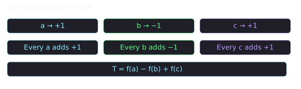
::: {.card-orange}
Every occurrence of the same value uses the same sign.
:::

## A signed counter

::: {.card-cyan}
Initialize $T=0$. On arrival of $s_t$, update
$$
T\gets T+b(s_t).
$$
At the end,
$$
T=\sum_{t=1}^m b(s_t)=\sum_{i=1}^n f_i b(i),\qquad X=T^2.
$$
:::

![](../figs/signs.svg){fig-alt="All occurrences of a key share one sign; their contributions add to a single signed counter." width=950}

## Expand the square

::: {.card-purple}
$$
T^2=\sum_i f_i^2b(i)^2+2\sum_{i<j}f_if_jb(i)b(j).
$$
:::

::: {.card-green}
The diagonal terms equal $f_i^2$; the cross terms have mean zero.
:::

## Pairwise independence gives the mean

::: {.card-cyan}
For $i\neq j$,
$$
\mathbb E[b(i)b(j)]=\mathbb E b(i)\mathbb E b(j)=0.
$$
Therefore
$$
\boxed{\mathbb E X=\mathbb E T^2=\sum_i f_i^2=F_2.}
$$
:::

## The variance requires four signs

::: {.card-purple}
$$
\mathbb E X^2=\mathbb E T^4
=\sum_{i,j,\ell,h} f_if_jf_\ell f_h
\mathbb E[b(i)b(j)b(\ell)b(h)].
$$
:::

::: {.card-cyan}
Classify quadruples by which indices repeat. There are at most four distinct signs in any term.
:::

## Terms with a singleton vanish

::: {.card-green}
If $i$ appears exactly once in a quadruple, independence gives
$$
\mathbb E[b(i)b(j)b(\ell)b(h)]
=\mathbb E b(i)\,\mathbb E[b(j)b(\ell)b(h)]=0.
$$
:::

::: {.card-orange}
This removes patterns $3+1$, $2+1+1$, and $1+1+1+1$.
:::

## Four equal indices survive

::: {.card-cyan}
For $(i,i,i,i)$,
$$
\mathbb E b(i)^4=1.
$$
The total contribution is
$$
\sum_i f_i^4=F_4.
$$
:::

## Two equal pairs survive

::: {.card-purple}
For each $i<j$, there are $\binom42=6$ orders of $(i,i,j,j)$.
$$
\mathbb E[b(i)^2b(j)^2]=1.
$$
Their total contribution is
$$
6\sum_{i<j}f_i^2f_j^2.
$$
:::

## Subtract the squared mean

::: {.card-green}
$$
\mathbb E T^4=F_4+6\sum_{i<j}f_i^2f_j^2,
\qquad F_2^2=F_4+2\sum_{i<j}f_i^2f_j^2.
$$
$$
\boxed{\operatorname{Var}(T^2)=4\sum_{i<j}f_i^2f_j^2\leq2F_2^2.}
$$
:::

## Store a seed, not all the signs

::: {.card-orange}
Keeping $n$ independent signs explicitly would use too much space.
:::

::: {.card-purple}
The notes use a random polynomial modulo a prime:
$$
g(x)=c_0+c_1x+\cdots+c_5x^5\pmod p.
$$
Choose independent uniform coefficients in $\mathbb F_p$, with $p>n$.
:::

## Why polynomial values are independent

::: {.card-green}
At $r\leq6$ distinct inputs, prescribed values impose $r$ independent linear equations on six coefficients.
$$
\Pr[g(i_1)=y_1,\ldots,g(i_r)=y_r]=p^{-r}.
$$
:::

::: {.card-cyan}
The Vandermonde matrix has full row rank: the inputs are distinct modulo $p$.
Six-wise independence is more than the four-wise independence needed here.
:::

## The polynomial construction has a zero output

::: {.card-purple}
For an odd prime $p$, define
$$
b(i)=\begin{cases}
0,&g(i)=p-1,\\
+1,&g(i)\text{ is odd},\\
-1,&g(i)\text{ is even and }g(i)\neq p-1.
\end{cases}
$$
:::

::: {.card-orange}
Keep these zero outputs. Conditioning on their absence need not preserve independence.
:::

## Normalize the ternary sketch

::: {.card-cyan}
Let $q=(p-1)/p\geq2/3$. Unconditionally,
$$
\mathbb E b(i)=0,\qquad
\mathbb E b(i)^2=\mathbb E b(i)^4=q.
$$
:::

::: {.card-green}
$$
T=\sum_i f_i b(i),\qquad X=\frac{T^2}{q},
\qquad \mathbb E X=F_2.
$$
:::

## Repeat the fourth-moment calculation

::: {.card-purple}
Singleton terms still vanish. The surviving terms give
$$
\mathbb E T^4=qF_4+6q^2\sum_{i<j}f_i^2f_j^2.
$$
Thus
$$
\mathbb E X^2=\frac1q F_4+6\sum_{i<j}f_i^2f_j^2.
$$
:::

## The same variance bound survives

::: {.card-green}
$$
\begin{aligned}
\operatorname{Var}(X)
&=(1/q-1)F_4+4\sum_{i<j}f_i^2f_j^2\\
&=2F_2^2+(1/q-3)F_4\\
&\leq2F_2^2.
\end{aligned}
$$
:::

::: {.card-cyan}
Since $q\geq2/3$, the coefficient $1/q-3$ is nonpositive.
:::

## Space and updates for one sketch

::: {.card-purple}
Choose a common odd prime $n<p=O(\max\{n,2\})$.
Store six coefficients and one signed counter.
:::

::: {.card-green}
$$
\text{seed: }O(\log(n+1))\text{ bits},\qquad |T|\leq m.
$$
Horner evaluation of the fixed-degree polynomial uses $O(1)$ modular operations per item.
:::

::: {.notes}
Use the word-RAM model with unit-cost arithmetic on a constant number of
words. Prime selection is preprocessing. Independent sketches have independent
coefficient vectors; sharing the fixed prime is harmless.
:::

## Average enough $F_2$ sketches

::: {.card-cyan}
$$
\alpha=\left\lceil16/\varepsilon^2\right\rceil,
\qquad A_i=\frac1\alpha\sum_{j=1}^{\alpha}X_{i,j}.
$$
$$
\Pr[|A_i-F_2|>\varepsilon F_2]
\leq\frac{2}{\alpha\varepsilon^2}\leq\frac18.
$$
:::

## Bound the number of bad blocks

::: {.card-purple}
Let $U=\sum_{i=1}^{\beta}\mathbf1[A_i\text{ is bad}]$ for independent blocks.
$$
\mathbb E[7^U]
=\prod_i\mathbb E[7^{\mathbf1[A_i\text{ bad}]}]
\leq(1+6/8)^\beta.
$$
:::

::: {.card-green}
$$
\Pr[U\geq\beta/2]\leq\frac{(7/4)^\beta}{7^{\beta/2}}
=\left(\frac{\sqrt7}{4}\right)^\beta\leq e^{-\beta/4}.
$$
:::

## Take the median

::: {.card-cyan}
Choose $\beta=2\lceil2\ln(1/\delta)\rceil+1$ and return
$$
\widehat F_2=\operatorname{median}(A_1,\ldots,A_\beta).
$$
$$
\Pr[|\widehat F_2-F_2|>\varepsilon F_2]
\leq\Pr[U\geq\beta/2]\leq\delta.
$$
:::

## The $F_2$ streaming theorem

::: {.card-green}
One pass, arbitrary fixed insertion-only stream, $0<\varepsilon,\delta<1$:
$$
\Pr[(1-\varepsilon)F_2\leq\widehat F_2\leq(1+\varepsilon)F_2]\geq1-\delta.
$$
$$
\boxed{O\left(\varepsilon^{-2}\log\frac2\delta\right)
\text{ words and time per item}.}
$$
:::

::: {.notes}
End the signed-sketch segment near minute 70. The theorem includes the
finite-seed implementation, not just the ideal-sign analysis.
:::

## Compare the two constructions

::: {.card-purple}
| | Reservoir differences | Signed sum |
|:---|:---|:---|
| Target | $F_k$, fixed $k\geq1$ | $F_2$ |
| Basic output | $m(r^k-(r-1)^k)$ | $T^2/q$ |
| Relative variance bound | $kn^{1-1/k}$ | $2$ |
| State per sketch | Representative and counter | Seed and counter |
:::

::: {.card-green}
Both use the same averaging and median framework.
:::

## Reconstruct the proof

::: {.card-cyan}
1. Why must reservoir replacement reset the suffix counter?
2. Where does the factor $n^{1-1/k}$ enter?
3. Why are two-wise independent signs enough for the mean, but four-wise independence is used for the variance?
4. What changes when the polynomial output may be zero?
:::

::: {.notes}
Allow board discussion in the final five minutes. Answers: suffix begins at
the newly sampled occurrence; the convexity bound on m; fourth-order products;
retain zeros and divide T squared by q.
:::

## Source and takeaways

::: {.card-green}
$$
\text{unbiased sketch}\ \longrightarrow\ \text{relative variance bound}
\ \longrightarrow\ \text{average and median}.
$$
:::

::: {.card-purple}
Based on Notes 28, *Frequency Estimation over a Stream*.
The frequency-moment results are attributed there to Alon, Matias, and Szegedy [@ams-scafm-99].

Prerequisite background: [@mr-ra-95].
:::

## References {.small}

::: {#refs}
:::