Frequency Estimation over a Stream

Notes 28 · Full lecture · 75 minutes

Sariel Har-Peled

CS 574 · University of Illinois, Urbana-Champaign · Fall 2026

Three steps to a streaming estimate

Build → analyze → amplify

An unbiased random variable is the starting point. Control its variance, average independent copies, then take a median.

Part Minutes
Model and frequency moments 5
Averaging and median amplification 15
A reservoir estimator for \(F_k\) 25
A smaller sketch for \(F_2\) 25
Guarantees and discussion 5

The stream and its frequency vector

\[ \sigma=(s_1,\ldots,s_m),\qquad s_t\in[n]=\{1,\ldots,n\}. \] \[ f_i=|\{t:s_t=i\}|,\qquad \sum_{i=1}^n f_i=m. \] \(m\) counts positions; \(n\) is the universe size.

One pass through an insertion-only stream; memory much smaller than a full frequency table.

Frequency moments

\[ F_k=\sum_{i=1}^n f_i^k. \] \[ F_0=|\{i:f_i>0\}|,\quad F_1=m,\quad F_2=\sum_i f_i^2,\quad F_\infty=\max_i f_i. \] For \(F_0\), use \(0^0=0\) and \(a^0=1\) for \(a>0\).

Today: \(F_k\) for fixed integer \(k\geq1\), then a better bound for \(F_2\).

What does a successful estimate mean?

For \(0<\varepsilon,\delta<1\), return \(\widehat F_k\) satisfying \[ \Pr\bigl[|\widehat F_k-F_k|>\varepsilon F_k\bigr]\leq\delta. \] The probability is over the algorithm’s randomness, for any fixed stream.

Words hold an item identifier or a stream counter. For fixed \(k\), a constant number of words also holds the needed powers. An empty stream is handled separately: return \(0\).

Unbiased is not yet accurate

The coin example

\[ X\sim\operatorname{Bernoulli}(p),\qquad \mathbb E X=p, \qquad \operatorname{Var}(X)=p(1-p). \] One flip returns \(0\) or \(1\), even when the target is a small positive \(p\).

We need a bound on deviation from the mean, not just the correct mean.

The abstract estimation problem

\[ \mathbb E X=\mu>0,\qquad \operatorname{Var}(X)=\nu<\infty. \] Construct \(Z\) with \[ \Pr[(1-\varepsilon)\mu\leq Z\leq(1+\varepsilon)\mu]\geq1-\delta. \]

The useful quantity is the relative variance \(\nu/\mu^2\).

Chebyshev sets the variance target

For any \(a>0\), \[ \Pr[|W-\mathbb E W|\geq a] \leq\frac{\operatorname{Var}(W)}{a^2}. \] If \(\mathbb E W=\mu\) and \(\operatorname{Var}(W)\leq\varepsilon^2\mu^2/4\), then \[ \Pr[|W-\mu|\geq\varepsilon\mu]\leq\frac14. \]

Average independent samples

\[ X_1,\ldots,X_\alpha\text{ independent copies of }X, \qquad A=\frac1\alpha\sum_{j=1}^\alpha X_j. \] \[ \mathbb E A=\frac1\alpha\sum_j\mathbb E X_j=\mu. \]

Averaging preserves the target mean.

Independence reduces variance

\[ \begin{aligned} \operatorname{Var}(A) &=\frac1{\alpha^2}\operatorname{Var}\left(\sum_jX_j\right)\\ &=\frac1{\alpha^2}\sum_j\operatorname{Var}(X_j) =\frac\nu\alpha. \end{aligned} \]

Repeatedly using the same random sample would not reduce variance.

Choose the block size

\[ \alpha=\max\left\{1,\left\lceil\frac{4\nu}{\varepsilon^2\mu^2}\right\rceil\right\}. \] \[ \Pr[|A-\mu|\geq\varepsilon\mu] \leq\frac\nu{\alpha\varepsilon^2\mu^2}\leq\frac14. \]

If \(\nu=0\), one sample is already exact. In an algorithm, a known upper bound on \(\nu/\mu^2\) suffices.

Why a second layer?

Chebyshev applied to one average of \(M\) samples gives \[ \Pr[\text{failure}]\leq\frac\nu{M\varepsilon^2\mu^2}. \] This route uses \(M\geq\nu/(\delta\varepsilon^2\mu^2)\) for failure \(\delta\).

The median of independent averages needs only logarithmically many blocks in \(1/\delta\).

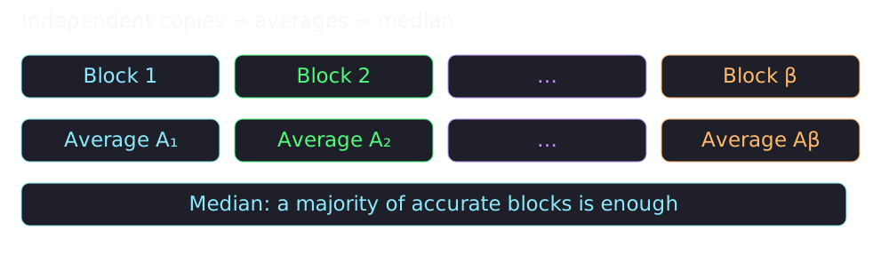
Median of averages

\[ A_i=\frac1\alpha\sum_{j=1}^\alpha X_{i,j},\qquad Z=\operatorname{median}(A_1,\ldots,A_\beta). \] All \(\alpha\beta\) samples are independent; take \(\beta\) odd.

Independent blocks are averaged; their averages feed one median.

A majority inside the interval traps the median

Let \(I=[(1-\varepsilon)\mu,(1+\varepsilon)\mu]\). \[ G_i=\mathbf1[A_i\in I],\qquad G=\sum_{i=1}^{\beta}G_i. \] \[ \Pr[G_i=1]\geq\frac34,\qquad \mathbb E G\geq\frac{3\beta}{4}. \]

\[ G>\beta/2\ \Longrightarrow\ Z\in I. \] A bad median therefore implies \(G<\beta/2\).

Chernoff bounds the bad majority

For independent Bernoulli variables and \(0<t<1\), \[ \Pr[G<(1-t)\mathbb E G]\leq e^{-t^2\mathbb E G/2}. \] Since \(\beta/2\leq(2/3)\mathbb E G\), \[ \Pr[Z\notin I]\leq e^{-\mathbb E G/18}\leq e^{-\beta/24}. \]

A complete amplification theorem

Choose \[ \alpha=\max\{1,\lceil4\nu/(\varepsilon^2\mu^2)\rceil\}, \qquad \beta=2\lceil12\ln(1/\delta)\rceil+1. \] Using \(M=\alpha\beta\) independent samples, \[ \Pr[|Z-\mu|>\varepsilon\mu]\leq\delta. \]

\[ M=O\left(\left(1+\frac\nu{\varepsilon^2\mu^2}\right) \log\frac2\delta\right). \] Compute block averages and select their median in \(O(M)\) time.

Return to the stream

Goal: one constant-size random sketch \(X\) with \(\mathbb E X=F_k\).

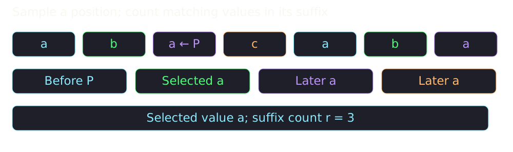
Pick a uniformly random stream position \(P\in[m]\). Store its value and count its occurrences from position \(P\) onward.

A random position, not a random distinct value

\[ \Pr[P=t]=1/m,\qquad \Pr[s_P=i]=f_i/m. \] Frequent values are more likely to be selected.

A stream with a selected occurrence; only equal values in the suffix contribute to the counter.

Reservoir sampling implements that choice

At position \(t\), replace the representative with \(s_t\) with probability \(1/t\).

For a fixed position \(p\leq m\), \[ \Pr[P=p]=\frac1p\prod_{t=p+1}^m\left(1-\frac1t\right) =\frac1p\cdot\frac pm=\frac1m. \] The final position is uniform without knowing \(m\) in advance.

Maintain the suffix count

State: position counter \(t\), representative \(v\), suffix counter \(r\).

On arrival of \(s_t\):

  1. With probability \(1/t\), set \(v\gets s_t\) and \(r\gets1\).
  2. Otherwise, if \(s_t=v\), set \(r\gets r+1\).

Replacement resets \(r\) even when the new representative has the same value.
What does the final counter represent?

If the final selected position is \(P\), then \[ r=|\{t\geq P:s_t=s_P\}|. \] For a value appearing \(f_i\) times, the suffix ranks at its occurrences are \[ f_i,f_i-1,\ldots,1. \]

Use a discrete derivative

\[ \Delta_k(r)=r^k-(r-1)^k,\qquad X=m\Delta_k(r). \]

\[ \sum_{r=1}^{f_i}\Delta_k(r)=f_i^k-0^k=f_i^k. \] The difference is chosen so the expectation telescopes.

Unbiasedness: sum over all positions

\[ \begin{aligned} \mathbb E X &=\frac1m\sum_{i=1}^n\sum_{r=1}^{f_i}m\Delta_k(r)\\ &=\sum_{i=1}^n\sum_{r=1}^{f_i}\bigl(r^k-(r-1)^k\bigr)\\ &=\sum_{i=1}^n f_i^k=F_k. \end{aligned} \]

Check the first moment

For \(k=1\), \[ X=m\bigl(r-(r-1)\bigr)=m=F_1. \] The estimator is deterministic and exact.

The interesting variance analysis begins at \(k>1\).

Check the second moment estimator

For \(k=2\), \[ X=m\bigl(r^2-(r-1)^2\bigr)=m(2r-1). \] For a value of frequency \(f\), \[ 1+3+\cdots+(2f-1)=f^2. \]

The telescoping idea is more general

Let \(g(0)=0\), and set \[ X_g=m\bigl(g(r)-g(r-1)\bigr). \] Then \[ \mathbb E X_g=\sum_{i=1}^n g(f_i). \]

This establishes the mean. A useful approximation still needs a variance bound.

Bound one increment

For \(r\geq1\) and \(k\geq1\), \[ 0\leq\Delta_k(r)=\int_{r-1}^r kx^{k-1}\,dx\leq kr^{k-1}. \]

For \(1\leq r\leq f\), \[ \Delta_k(r)^2\leq kf^{k-1}\Delta_k(r). \]

Sum the squared increments

\[ \begin{aligned} \sum_{r=1}^{f}\Delta_k(r)^2 &\leq kf^{k-1}\sum_{r=1}^{f}\Delta_k(r)\\ &=kf^{k-1}f^k=kf^{2k-1}. \end{aligned} \]

One factor is bounded; the other still telescopes.

The probabilistic second moment

\[ \begin{aligned} \mathbb E X^2 &=m\sum_{i=1}^n\sum_{r=1}^{f_i}\Delta_k(r)^2\\ &\leq km\sum_i f_i^{2k-1} =kmF_{2k-1}. \end{aligned} \]

We need to compare this with \(F_k^2\).

Compare the first and \(k\)th moments

Convexity of \(x\mapsto x^k\) gives \[ \left(\frac1n\sum_i f_i\right)^k \leq\frac1n\sum_i f_i^k. \] Taking \(k\)th roots, \[ \boxed{m\leq n^{1-1/k}F_k^{1/k}.} \]

Bound the largest frequency

Let \(L=\max_i f_i\). Then \[ L^k\leq\sum_i f_i^k=F_k, \qquad L^{k-1}\leq F_k^{(k-1)/k}. \]

\[ F_{2k-1}=\sum_i f_i^k f_i^{k-1}\leq L^{k-1}F_k. \]

Compare the higher moment with \(F_k\)

\[ F_{2k-1}\leq F_k^{(k-1)/k}F_k=F_k^{(2k-1)/k}. \] Multiply by the bound on \(m\): \[ \boxed{mF_{2k-1}\leq n^{1-1/k}F_k^2.} \]

The relative variance bound

\[ \begin{aligned} \operatorname{Var}(X) &=\mathbb E X^2-F_k^2\\ &\leq kmF_{2k-1}\\ &\leq kn^{1-1/k}F_k^2. \end{aligned} \] \[ \boxed{\frac{\operatorname{Var}(X)}{(\mathbb E X)^2}\leq kn^{1-1/k}.} \]

Choose parameters before the stream arrives

\[ \alpha=\left\lceil\frac{4kn^{1-1/k}}{\varepsilon^2}\right\rceil, \qquad\beta=2\lceil12\ln(1/\delta)\rceil+1. \] Run \(\alpha\beta\) independent reservoir sketches on the same stream.

These parameters use the known bound on relative variance. They do not require knowing \(F_k\).

General-moment theorem

For fixed integer \(k\geq1\), a one-pass algorithm returns \(\widehat F_k\) with \[ \Pr[|\widehat F_k-F_k|>\varepsilon F_k]\leq\delta \] using \[ O\left(kn^{1-1/k}\varepsilon^{-2}\log\frac2\delta\right) \quad\text{words}. \]

The direct implementation performs one constant-time update per sketch per item.

Why specialize to \(F_2\)?

Substituting \(k=2\) gives \[ O\left(\sqrt n\,\varepsilon^{-2}\log\frac2\delta\right) \quad\text{words}. \]

Random signs give relative variance at most \(2\), removing the \(\sqrt n\) factor.

Assign randomness to values

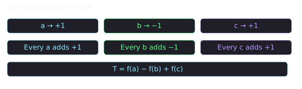
For now, let \(b(1),\ldots,b(n)\in\{-1,+1\}\) be unbiased, four-wise independent signs. \[ \mathbb E b(i)=0,\qquad b(i)^2=1. \]

Every occurrence of the same value uses the same sign.

A signed counter

Initialize \(T=0\). On arrival of \(s_t\), update \[ T\gets T+b(s_t). \] At the end, \[ T=\sum_{t=1}^m b(s_t)=\sum_{i=1}^n f_i b(i),\qquad X=T^2. \]

All occurrences of a key share one sign; their contributions add to a single signed counter.

Expand the square

\[ T^2=\sum_i f_i^2b(i)^2+2\sum_{i<j}f_if_jb(i)b(j). \]

The diagonal terms equal \(f_i^2\); the cross terms have mean zero.

Pairwise independence gives the mean

For \(i\neq j\), \[ \mathbb E[b(i)b(j)]=\mathbb E b(i)\mathbb E b(j)=0. \] Therefore \[ \boxed{\mathbb E X=\mathbb E T^2=\sum_i f_i^2=F_2.} \]

The variance requires four signs

\[ \mathbb E X^2=\mathbb E T^4 =\sum_{i,j,\ell,h} f_if_jf_\ell f_h \mathbb E[b(i)b(j)b(\ell)b(h)]. \]

Classify quadruples by which indices repeat. There are at most four distinct signs in any term.

Terms with a singleton vanish

If \(i\) appears exactly once in a quadruple, independence gives \[ \mathbb E[b(i)b(j)b(\ell)b(h)] =\mathbb E b(i)\,\mathbb E[b(j)b(\ell)b(h)]=0. \]

This removes patterns \(3+1\), \(2+1+1\), and \(1+1+1+1\).

Four equal indices survive

For \((i,i,i,i)\), \[ \mathbb E b(i)^4=1. \] The total contribution is \[ \sum_i f_i^4=F_4. \]

Two equal pairs survive

For each \(i<j\), there are \(\binom42=6\) orders of \((i,i,j,j)\). \[ \mathbb E[b(i)^2b(j)^2]=1. \] Their total contribution is \[ 6\sum_{i<j}f_i^2f_j^2. \]

Subtract the squared mean

\[ \mathbb E T^4=F_4+6\sum_{i<j}f_i^2f_j^2, \qquad F_2^2=F_4+2\sum_{i<j}f_i^2f_j^2. \] \[ \boxed{\operatorname{Var}(T^2)=4\sum_{i<j}f_i^2f_j^2\leq2F_2^2.} \]

Store a seed, not all the signs

Keeping \(n\) independent signs explicitly would use too much space.

The notes use a random polynomial modulo a prime: \[ g(x)=c_0+c_1x+\cdots+c_5x^5\pmod p. \] Choose independent uniform coefficients in \(\mathbb F_p\), with \(p>n\).

Why polynomial values are independent

At \(r\leq6\) distinct inputs, prescribed values impose \(r\) independent linear equations on six coefficients. \[ \Pr[g(i_1)=y_1,\ldots,g(i_r)=y_r]=p^{-r}. \]

The Vandermonde matrix has full row rank: the inputs are distinct modulo \(p\). Six-wise independence is more than the four-wise independence needed here.

The polynomial construction has a zero output

For an odd prime \(p\), define \[ b(i)=\begin{cases} 0,&g(i)=p-1,\\ +1,&g(i)\text{ is odd},\\ -1,&g(i)\text{ is even and }g(i)\neq p-1. \end{cases} \]

Keep these zero outputs. Conditioning on their absence need not preserve independence.

Normalize the ternary sketch

Let \(q=(p-1)/p\geq2/3\). Unconditionally, \[ \mathbb E b(i)=0,\qquad \mathbb E b(i)^2=\mathbb E b(i)^4=q. \]

\[ T=\sum_i f_i b(i),\qquad X=\frac{T^2}{q}, \qquad \mathbb E X=F_2. \]

Repeat the fourth-moment calculation

Singleton terms still vanish. The surviving terms give \[ \mathbb E T^4=qF_4+6q^2\sum_{i<j}f_i^2f_j^2. \] Thus \[ \mathbb E X^2=\frac1q F_4+6\sum_{i<j}f_i^2f_j^2. \]

The same variance bound survives

\[ \begin{aligned} \operatorname{Var}(X) &=(1/q-1)F_4+4\sum_{i<j}f_i^2f_j^2\\ &=2F_2^2+(1/q-3)F_4\\ &\leq2F_2^2. \end{aligned} \]

Since \(q\geq2/3\), the coefficient \(1/q-3\) is nonpositive.

Space and updates for one sketch

Choose a common odd prime \(n<p=O(\max\{n,2\})\). Store six coefficients and one signed counter.

\[ \text{seed: }O(\log(n+1))\text{ bits},\qquad |T|\leq m. \] Horner evaluation of the fixed-degree polynomial uses \(O(1)\) modular operations per item.

Average enough \(F_2\) sketches

\[ \alpha=\left\lceil16/\varepsilon^2\right\rceil, \qquad A_i=\frac1\alpha\sum_{j=1}^{\alpha}X_{i,j}. \] \[ \Pr[|A_i-F_2|>\varepsilon F_2] \leq\frac{2}{\alpha\varepsilon^2}\leq\frac18. \]

Bound the number of bad blocks

Let \(U=\sum_{i=1}^{\beta}\mathbf1[A_i\text{ is bad}]\) for independent blocks. \[ \mathbb E[7^U] =\prod_i\mathbb E[7^{\mathbf1[A_i\text{ bad}]}] \leq(1+6/8)^\beta. \]

\[ \Pr[U\geq\beta/2]\leq\frac{(7/4)^\beta}{7^{\beta/2}} =\left(\frac{\sqrt7}{4}\right)^\beta\leq e^{-\beta/4}. \]

Take the median

Choose \(\beta=2\lceil2\ln(1/\delta)\rceil+1\) and return \[ \widehat F_2=\operatorname{median}(A_1,\ldots,A_\beta). \] \[ \Pr[|\widehat F_2-F_2|>\varepsilon F_2] \leq\Pr[U\geq\beta/2]\leq\delta. \]

The \(F_2\) streaming theorem

One pass, arbitrary fixed insertion-only stream, \(0<\varepsilon,\delta<1\): \[ \Pr[(1-\varepsilon)F_2\leq\widehat F_2\leq(1+\varepsilon)F_2]\geq1-\delta. \] \[ \boxed{O\left(\varepsilon^{-2}\log\frac2\delta\right) \text{ words and time per item}.} \]

Compare the two constructions

Reservoir differences Signed sum
Target \(F_k\), fixed \(k\geq1\) \(F_2\)
Basic output \(m(r^k-(r-1)^k)\) \(T^2/q\)
Relative variance bound \(kn^{1-1/k}\) \(2\)
State per sketch Representative and counter Seed and counter

Both use the same averaging and median framework.

Reconstruct the proof

  1. Why must reservoir replacement reset the suffix counter?
  2. Where does the factor \(n^{1-1/k}\) enter?
  3. Why are two-wise independent signs enough for the mean, but four-wise independence is used for the variance?
  4. What changes when the polynomial output may be zero?

Source and takeaways

\[ \text{unbiased sketch}\ \longrightarrow\ \text{relative variance bound} \ \longrightarrow\ \text{average and median}. \]

Based on Notes 28, Frequency Estimation over a Stream. The frequency-moment results are attributed there to Alon, Matias, and Szegedy (Alon, Matias, & Szegedy, 1999).

Prerequisite background: (Motwani & Raghavan, 1995).

References

Alon, N., Matias, Y., & Szegedy, M. (1999). The space complexity of approximating the frequency moments. J. Comput. Syst. Sci., 58(1), 137–147. https://doi.org/10.1006/jcss.1997.1545
Motwani, R., & Raghavan, P. (1995). Randomized algorithms. Cambridge University Press. https://doi.org/10.1017/cbo9780511814075