Since this class depends on data structures, which has discrete math as a prerequisite, most people have probably seen some version of BFS, DFS, and state graphs before. If this isn't true for you, this lecture probably went too fast. Aside from the textbook, you may wish to browse web pages for CS 173, CS 225, and/or web tutorials on BFS/DFS.
A state graph has the following key parts:
The task is to find a lowest-cost path from start state to a goal state. Or, in some cases, a path whose cost is close to lowest cost. A major challenge in AI search is that the search spaces are often very large.
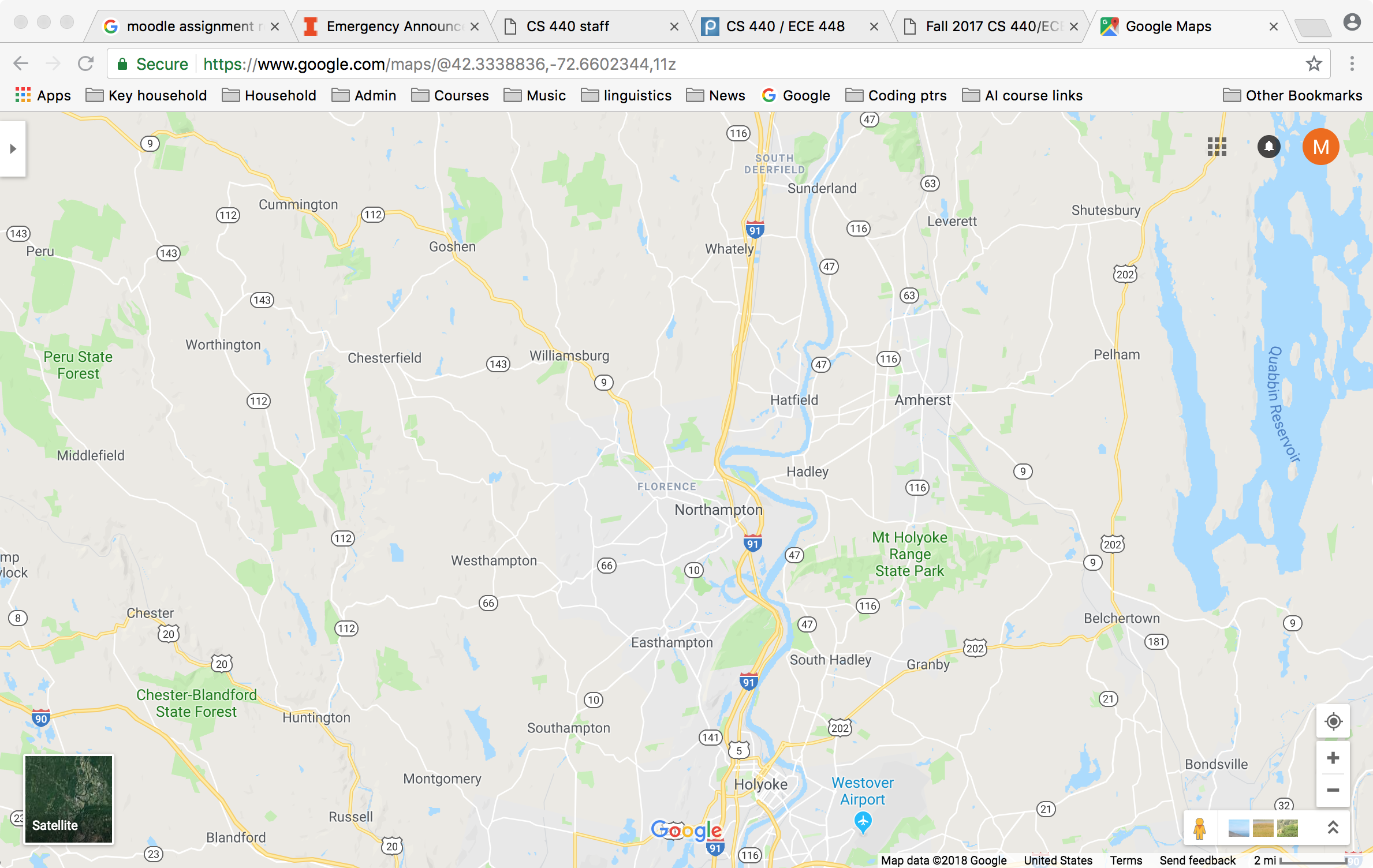
For example, consider the Missionaries and Cannibals puzzle. In the starting state, there are three missionaries, three cannibals, and a boat on the left side of a river. We need to move all six people to the right side, subject to the following constraints:
The state of the world can be described by three variables: how many missionaries on the left bank, how many cannibals on the left bank, and which bank the boat is on. The state space is shown below:
(from Gerhard Wickler, U. Edinburgh)
In this example, the states are sets of values for the three variables. The actions involve loading or unloading people from the boat and moving the boat across the river. The edge costs are constant.
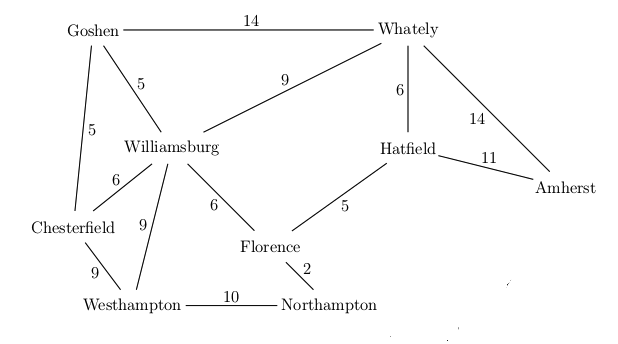
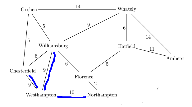
We can take a real-world map (below left) and turn it into a graph (below right). Notice that the graph is not even close to being a tree. So search algorithms have to actively prevent looping, e.g. by remember which locations they've already visited.
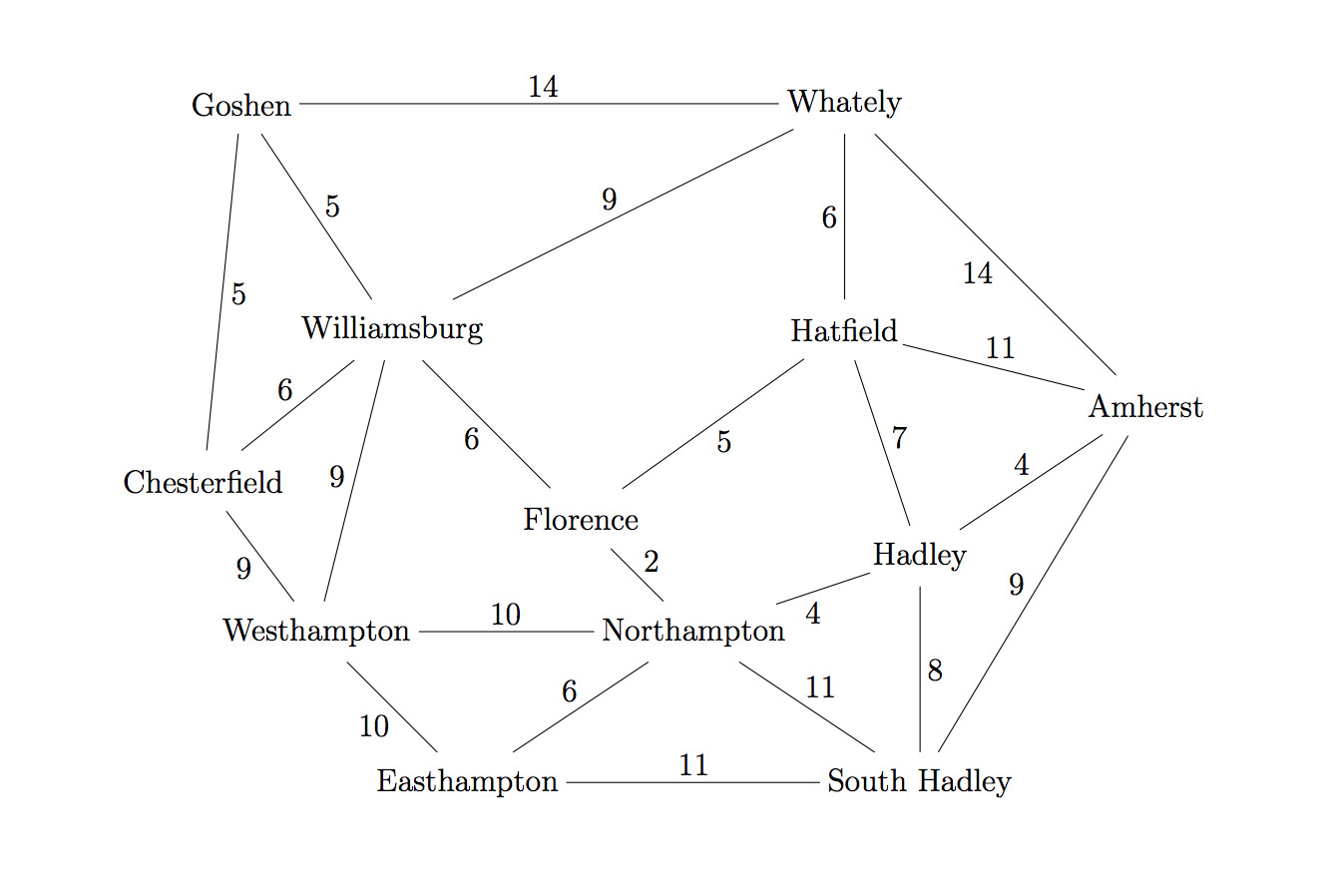
Mapping this onto a state graph:
On the graph, it's easy to see that there are many paths from Northampton to Amherst, e.g. 8 miles via Hadley, 31 miles via Williamsburg and Whately.
Each state in a search problem must contain all the information about the world that is relevant to defining and reaching the goal. The agent's geographic location is frequently not enough. Suppose you're playing an adventure game. These two states aren't the same, and getting from the first to the second constitutes significant progress towards winning the game.
Similarly, these two states differ significantly if you need to cross the river:
Our search will use two main data structures:
Basic outline for search code
Loop until you find a goal state or queue is empty
- pop state S off frontier
- follow outgoing edges to find S's neighbors
- for each neighbor X that has not yet been visited
- add X to the visited table and to the frontier
Our data structure for storing the frontier determines the type of search
"Follow outgoing edges" may mean literally traversing edges in a pre-built graph data structure. However, in an AI context it often means dynamically constructing the list of neighboring states.
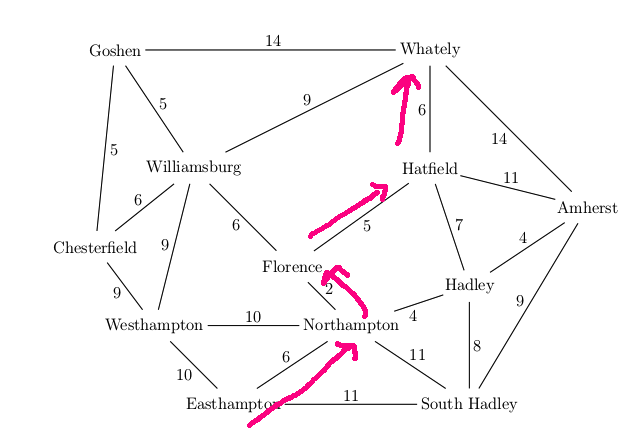
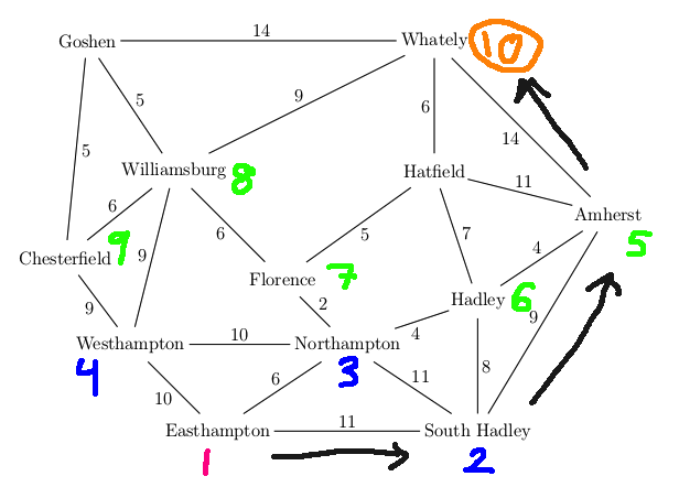
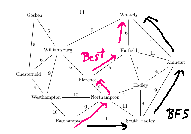
Let's find a route from Easthampton to Whately in our example map. The actual best route is via Northampton, Florence, Hatfield (19 miles)
Breadth-first search treats all edges as having the same cost. That is, it returns a path that uses the minimum number of edges. The frontier is implemented as a (FIFO) queue, in which shorter paths will end up in front of longer ones. So we explore locations in rings, gradually moving outwards from the starting location.
Let's use BFS to find a route from Easthampton to Whately and let's suppose that the outgoing edges for each town are stored in counterclockwise order.
A trace of the algorithm looks like this:
We return the path Easthampton, South Hadley, Amherst, Whately (length 34). This isn't the shortest path by mileage, but it's one of the shortest paths measured by number of edges.
The main loop for BFS looks like this:
Loop until queue is empty
- pop state S off frontier
- follow outgoing edges to find S's neighbors
- for each neighbor X that has not yet been visited
- If X is a goal state, halt and return its path
- Otherwise, add X to the visited table and to the frontier
The search can return as soon as a goal state is visited, i.e. when we'd normally put that state into the visited states table. (Note that this is NOT the same as UCS and \(A^*\) search below.) Do not wait until the queue is empty.
Properties:
Here is a fun animation of BFS set to music.
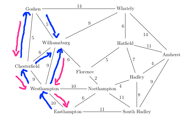
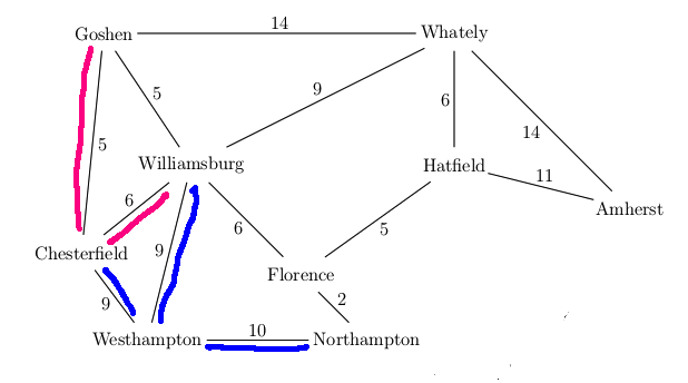
When a search algorithm finds the goal, it must be able to return the best path to the goal. To be able to retrieve this path efficiently at the end, the table of visited states will store a "backpointer" from each state to the previous state in its best path. When the goal is found, we retrieve the best path by chaining backwards using the backpointers until we reach the start state.
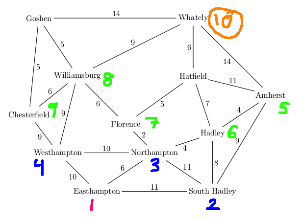
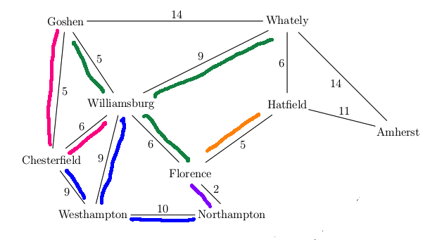
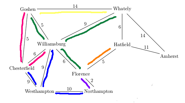
For example, suppose that our search algorithm has started from Easthampton and has explored all the blue edges in the map below. For each town, there is a best path back to Easthampton using only the edges explored so far (blue edges). For example, the best path for Williamsburg is via Westhampton. We've also seen a route to Williamsburg via Chesterfield and another via Goshen, but these are both longer. So the backpointer for Williamsburg (in red) goes to Westhampton. When we've seen two routes of the same length, you can pick either when storing the backpointer.
Breadth-first search returns a path that uses the fewest edges. However, this may not be the shortest path if you take edge costs into account. In the example below, the shortest path has length 19 and the BFS path has length 34.
Uniform-cost search (UCS) is a similar algorithm that finds optimal paths even when edge costs vary. To do this, we store the frontier using a priority queue. The priority of each state is the cost to reach it from the start state, i.e. the sum of the edges in the best path connecting it to the start state. The condition for stopping the search loop is slightly different from BFS: we return when a goal state is popped off the frontier.
Want to find best route from Westhampton to Hatfield in this simplified map
Our goal state is now at the front of the queue, so we're finished and can return this path.
A new feature in UCS search is that our first visit to a state may not be via the best path to that state. E.g. in the above example, we had to update the distance to Florence the second time we visited it. Therefore our table of visited states needs to store the distance to each state. When we find a better path to a previously-visited state, we need to
If the distance to a state needs to be updated, the state is guaranteed to be in the frontier. However, many efficient priority queue implementations do not support updates to the priorities. It's often best to simply put a new copy of the state (with its new cost) into the priority queue. In many applications, decreases in state cost aren't very frequent so this won't create very many duplicate states.
For related reasons, we cannot stop the search right away when we create a goal state. At that point, we've found one route to the goal, but perhaps not the best one. So we need to put the goal state back onto the frontier. We stop the search when the goal state reaches the top of the priority queue, i.e. when all states in the priority queue have a distance that is at least as large as the goal state.
So the main loop for UCS looks like this
Loop until queue is empty
- pop state S off frontier
- if S is a goal state, halt and return path
- follow outgoing edges to find its S's neighbors
- for each neighbor state X,
- if X is in the visited table but we've found a shorter path to it, update the visited table and push a new copy of X onto the frontier
- if X is not in the visited table, add it to the visited table and frontier
To do the analysis right, we need to assume
These assumptions are almost always true in practical uses of these algorithms. If they aren't true, algorithm design and analysis can get much harder in ways that are beyond the scope of this class.
Given those assumptions, UCS returns an optimal path even if edge costs vary. Memory requirements for UCS are similar to BFS. They can be worse than BFS in some cases, because UCS can get stuck in extended areas of short edges rather than exploring longer but more promising edges.
You may have seen Dijkstra's algorithm in data structures class. It is basically similar to UCS, except that it finds the distance from the start to all states rather than stopping when it reaches a designated goal state.

Shakey the robot (1966-72), from Wired Magazine
\(A^*\) search was developed around 1968 as part of the Shakey project at Stanford. It's still a critical component of many AI systems. The Shakey project ran from 1966 to 1972. Here's some videos showing Shakey in action.
Towards the end of the project, it was using a PDP-10 with about 800K bytes of RAM. The programs occupied 1.35M of disk space. This kind of memory starvation was typical of the time. For example, the guidance computer for Apollo 11 (first moon landing) in 1969 had only 70K bytes of storage.
BFS and UCS prioritize search states based on the cost to reach each state from the start. This isn't a great predictor of how quickly a route will reach a goal. If you play around with this search technique demo by Xueqiao Xu, you can see that BFS and UCS ("Dijkstra") search a widening circular space, most of which is in the direction opposite to the goal. When they assess states, they consider only distance from the starting position, but not the distance to reach the goal.
Key idea: combine distance so far with an estimate of the remaining distance to the goal.
Our main search loop for \(A^*\) looks like the one for UCS. However, a state x's queue priority is an estimate f(x) of the final length of a path through that state to the goal. Specifically, f(x) is the sum of
With a reasonable choice of heuristic, \(A^*\) does a better job of directing its attention towards the goal. Try the search demo again, but select \(A^*\).
Heuristic functions for A* need to have two properties
"Underestimate" includes the possibility that the estimate is equal to the true distance. In the context of \(A^*\) search, being an underestimate is also known as being "admissible."
Heuristics are usually created by simplifying ("relaxing") the task, i.e. removing some constraints. For planning paths for a car or robot, we can use straight line distance. This ignores
All other things being equal, an admissible heuristic will work better if it is closer to the true cost, i.e. larger. A heuristic function h is said to "dominate" a heuristic function with lower values.
For example, suppose that driving in a classic Midwest city where all streets go north-south or east-west, never diagonally. Straight-line distance is still one possible \(A^*\) heuristic. However, a better heuristic is Manhattan distance. The Manhattan distance between two points is the difference in their x coordinates plus the difference in their y coordinates. Manhattan distance dominates straight-line distance. If there are also diagonal streets, we can't use Manhattan distance because it can overestimate the distance to the goal.
Another classical example for \(A^*\) is the 15-puzzle. A smaller variant of this is the 8-puzzle..
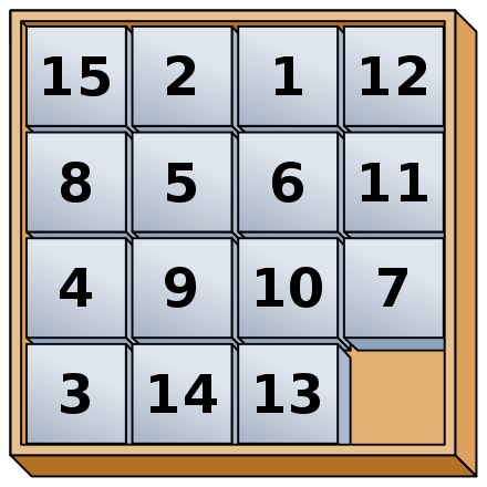
Two simple heuristics for the 15-puzzle are
Admissibility guarantees that the output solution is optimal. Here's a sketch of the proof:
Search stops when goal state becomes top option in frontier (not when goal is first discovered). Suppose we have found goal with path P and cost C. Consider a partial path X in the frontier. Its estimated cost must be \(\ge C\). Since our heuristic is admissible, the true cost of extending X to reach the goal must also be \( \ge C\). So extending X can't give us a better path than P.
Let's go back to the situation when UCS or \(A^*\) revisits a state via a shorter path. In that situation, we pushed a new copy of the state onto the (frontier) queue with the new improved priority. Suppose we're using a priority queue implementation that allows us to simply update the priority of a state in the queue. Are we guaranteed that the target state will still be in the queue or do we potentially need to reinsert the state into the queue?
For \(A^*\), the node we want to update is guaranteed to be in the queue if the heuristic is "consistent". Suppose that we can get from s to s' with cost c(s,s'). For a consistent heuristic, we must have:
\( h(s) \le c(s,s') + h(s') \)
That is, as we follow a path away from start state, our estimated cost f never decreases.
In practice, admissible heuristics are typically consistent. For example, the straight-line distance is consistent because of the triangle inequality. Uniform cost search is \(A^*\) with a heuristic function that always returns zero. That heuristic is consistnt. However, if you are writing general-purpose search code, it's best to use a method that will still work if the heuristic isn't consistent, such as pushing a duplicate copy of the state onto the queue.
Consistency implies admissibility, but not vice versa.
In case you are curious, the following highly artificial example shows a heuristic that's admissible but not consistent.
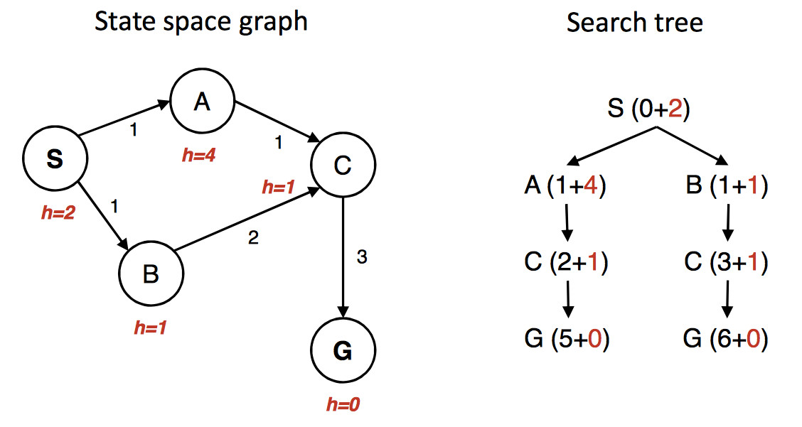
(from Berkeley CS 188x materials)
The state graph is shown on the left, with the h value under each state. The right shows a quick picture of the search process. Walking through the search in more detail:
First we put S in the queue with estimated cost 2, i.e. g(S) = 0 plus h(S) = 2.
We remove S from the queue and add its neighbors. A has estimated cost 5 and B has estimated cost 2. S is now done/closed.
We remove B from the queue and add its neighbor C. C has estimated cost 4. B is now done/closed.
We remove C from the queue. One of its neighbors (A) is already in the queue. So we only need to add G. G has cost 6. C is now done/closed.
We remove A from the queue. Its neighbors are all done, so we have nothing to do. A is now done.
We remove G from the queue. It's the goal, so we halt, reporting that the best path is SBCG with cost 6.
Oops. The best path is through A and has actual cost 5. But heuristic was admissible. What went wrong? We gave up too early on the node C. C had been removed from the queue before we found the shorter path to C. So we should have put C back onto the queue with its new updated cost.