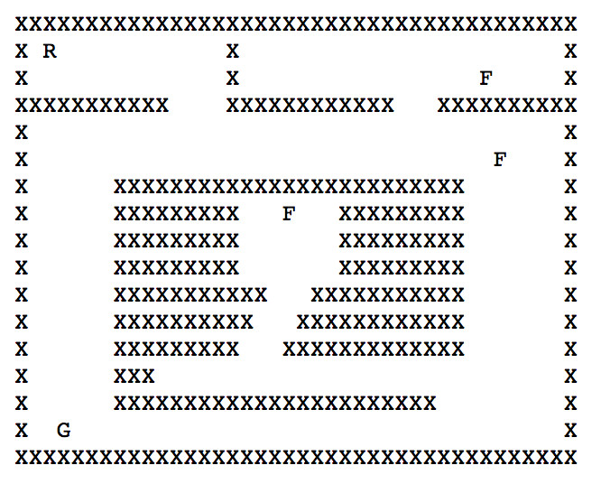
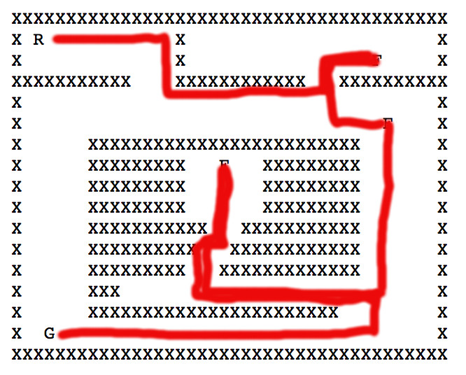
The picture below left shows an ASCII maze of the sort used in 1980's computer games. R is the robot, G is the goal, F is a food pellet to collect on the way to the goal. We no longer play games of this style, but you can still find search problems with this kind of simple structure. On the right is one path to the goal. Notice that it has to double back on itself in two places.
Modelling this as a state graph:
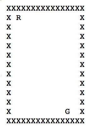
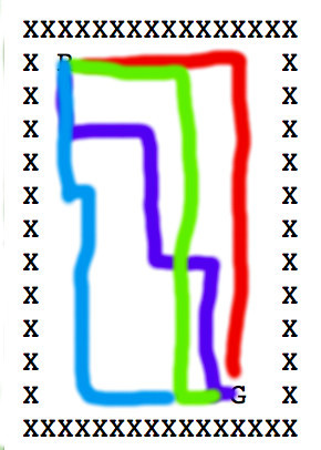
Some mazes impose tight constraints on where the robot can go, e.g. the bottom corridor in the above maze is only one cell wide. Mazes with large open areas can have vast numbers of possible solutions. For example, the maze below has many paths from start to goal. In this case, the robot needs to move 10 steps right and 10 steps down. Since there are no walls constraining the order of right vs. downward moves, there are \(20 \choose 10 \) paths of shortest length (20 steps), which is about 185,000 paths. We need to quickly choose one of these paths rather than wasting time exploring all of them individually.
One approach to this kind of exploding search space is to adjust the queue priorities so that one path has a slight edge over paths with identical real cost. The simplest approach involves adding an explicit tie-breaking step to the queue comparisons, so that a state created more recently will be ordered in the queue ahead of a state created earlier.
Alternatively, we can multiply our heuristic values by a factor slightly bigger than 1. This gives \(A*\) a small preference for extending the paths it's already working on, rather that exploring a wide set of very similar paths. This can speed up search significantly. The downside is that \(A*\) may return a path that isn't the shortest possible. Usually the path lengths remain close to optimal, so this type of "suboptimal" search is often a good choice in practice.
See Amit Patel's notes for details and related methods.
A good search algorithm must be coupled with a good representation of the problem. So transforming to a different state graph model may dramatically improve performance. We'll illustrate this with finding edit distance, and see other examples of good problem reformulation when we get to robot motion planning and classical planning.
Problem: find the best alignment between two strings, e.g. "ALGORITHM" and "ALTRUISTIC". By "best," we mean the alignment that requires the fewest editing operations (delete char, add char, substitute char) to transform the first word into the second. We can get from ALGORITHM to ALTRUISTIC with six edits, producing the following optimal alignment:
     A L G O R   I   T H M
     A L   T R U I S T I C
         D S   A   A   S S

D = delete character
A = add character
S = substitute
Versions of this task appear in
Each state is a string. So the start state would be "algorithm" and the end state is "altruistic." Each action applies one edit operation, anywhere in the word.
In this model, each state has a very large number of successors. So there are about \( 28^9 \) single-character changes you could make to ALGORITHM, resulting in words like:
    LGORITHM, AGORITHM, ..., ALGORIHM, ...
    BLGORITHM, CLGORITHM, ....
    AAGORITHM, ....
    ...
    ALBORJTHM, ...
    ....
This massive fan-out will cause search to be very slow.
A better representation for this problem explores the space of partial matches. Each state is an alignment of the initial sections (prefixes) of the two strings. So the start state is an alignment of two empty strings, and the end state is an alignment of the full strings.
In this representation, each action extends the alignment by one character. From each state, there are only three legal moves:
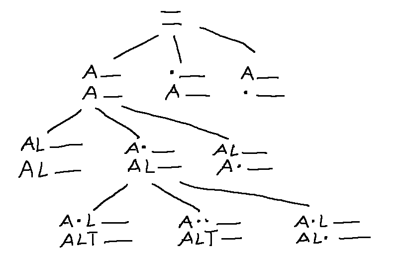
Here's part of the search tree, showing how we extend the alignment with each step. (A dot represents a skipped character.)
In this specific case, we can pack our work into a nifty compact 2D table.
This algorithm can be adapted for situations where the search space is too large to maintain the full alignment table. for example, we may need to match DNA sequences that are \(10^5\) characters long.
For more detail, see Wikipedia on edit distance and Jeff Erickson's notes.
In speech recognition, we need to transcribe an acoustic waveform into to produce written text. We'll see details of this process later in the course. For now, just notice that this proceeds word-by-word. So we have a set of candidate transcriptions for the first part of the waveform and wish to extend those by one more word. For example, one candidate transcription might start with "The book was very" and the acoustic matcher says that the next word sounds like "short" or "sort."
In this example
Speech recognition systems have vast state spaces. A recognition dictionary may know about 100,000 different words. Because acoustic matching is still somewhat error-prone, there may be many words that seem to match the next section of the input. So the currently-relevant states are constructed on demand, as we search.
In this situation, a common variation on \(A^*\) is "beam search". "Beam search" algorithms prune states with high values of f, frequently restricting the queue to some fixed length N. Like suboptimal search, this sabotages guarantees of optimality. However, in practice, it may be extremely unlikely that these poorly-rated states can be extended to a good solution.
Even in situations less extreme than speech recognition good implementations of \(A*\) and similar algorithms can require a lot of memory to store the visited table and the frontier. In some situations, we can reduce the memory footprint of search using depth-first search (DFS). In depth-first search, the frontier is stored as a stack (explicitly or implicitly via recursive function calls). So it fully extends the current path, i.e. the one represented by the state at the top of the stack, before moving on to other alternatives.
Here's an example of DFS in action. We'll explore each node's edges counterclockwise.
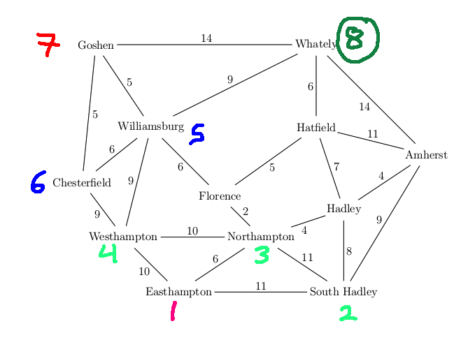
Detailed trace:
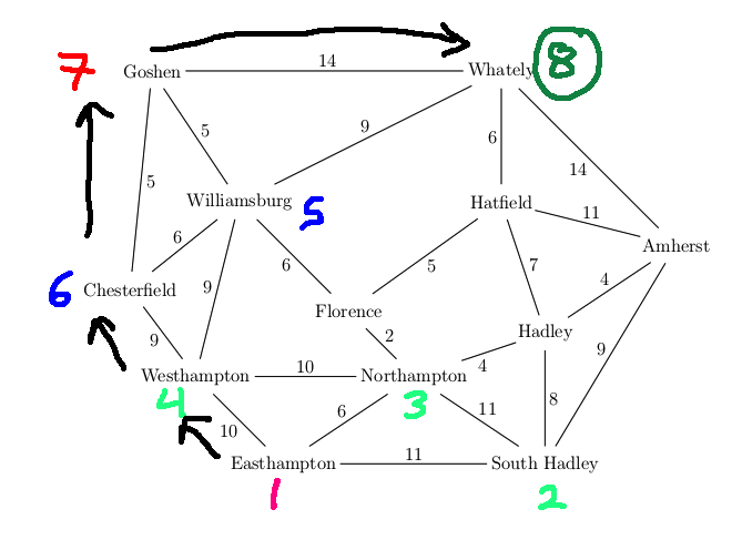
We return the path: Easthampton, Westhampton, Chesterfield, Goshen, Whately (length 38) Recall that the best path had length 19.
Animation of DFS set to music. Compare this to the one for BFS.
As you can see from the example, DFS can perform very poorly even on simple examples. If the search space is infinite (e.g. dynamically constructed), DFS is not guaranteed to reach the goal even if the goal is right near the start. If the frontier is implemented implicitly using recursion, DFS may hit system limits on the size of the recursion stack.
However, good implementations of DFS can be very efficient. So DFS can be useful when we have tight control of path length. Tight limits on path length can happen for three reasons:
Some of these situations also have tree-like search spaces, in which it's impossible to loop back to a state once we've visited it.
Suppose that DFS is limited to a short path length k ("length-bounded DFS"). That is, once the current path reaches length k without reaching a goal, we stop extending it. In most practical situations, the frontier for DFS has length roughly proportional to the length of the current path being explored. So bounding the path length also keeps the frontier small.
We still have to worry about the size of the table of visited states, which is used to prevent looping. Length-bounded DFS frequently omits that table, perhaps still checking that states do not repeat along the current path. So the search may end up duplicating some work because it forgets which states it has already explored, but the length bound keeps this inefficiency under control. However, with the frontier kept small and the visited state table omitted, the DFS implementation can be very efficient, in terms of both memory and speed.
Because of the need for a length bound, DFS is a niche technique, but one that can be very effective in the right situations.
We can dramatically improve the low-memory version of DFS by running it with a progressively increasing bound on the maximum path length. This is a bit like having a dog running around you on a leash, and gradually letting the leash out. Specifically:
For k = 1 to infinityRun DFS but stop whenever a path contains at least k states.
Halt when we find a goal state
This is called "iterative deepening." Its properties
Each iteration repeats the work of the previous one. So iterative deepening is most useful when the new search area at distance k is large compared to the area search in previous iterations, so that the search at distance k is dominated by the paths of length k.
These conditions don't hold for 2D mazes. The search area at radius k is proportional to k, whereas the area inside that radius is proportional to \(k^2\).
However, suppose that the search space looks like a 4-ary tree. We know from discrete math that there are \(4^k\) nodes at level k. Using a geometric series, we find that there are only \(1/3\cdot (4^k -1)\) nodes in levels 1 through k-1. So the nodes in the lowest level dominate the search. This type of situation holds (approximately) for big games such as chess.
Suppose that you need to move the robot (R) through multiple waypoints. It's tempting to use the following "greedy" method. You search for the closest waypoint. Then you launch a new search from that waypoint to find the next waypoint. And you keep going, each time looking for the nearest individual waypoint. So the top level of your code is a loop that repeatedly calls your search method (e.g. BFS or A*).
Greedy search does not always return optimal paths. For example, consider the example below. (The numbers are x coordinates.)
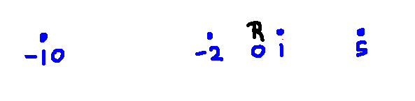
The greedy strategy will produce this path:
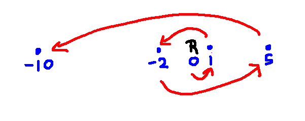
You should be able to find a much shorter path that goes through all the waypoints.
There are many other specialized variants of search algorithms.
Iterative deepening \(A^*\): Like iterative deepening, but using \(A^*\) rather than DFS. If the current bound is k, the search stops when the estimated total cost f(s) is larger than k.
Pattern databases: A pattern database is a database of partial problems, together with the cost to solve the partial problem. The true solution cost for a search state must be at least as high as the cost for any pattern it contains.
Backwards and bidirectional search : Basically what they sound like. Backwards search is like forwards search except that you start from the goal. In bidirectional search, you run two parallel searches, starting from start and goal states, in hopes that they will connect at a shared state. These approaches are useful only in very specific situations.
Backwards search makes sense when you have relatively few goal states, known at the start. This often fails, e.g. chess has a huge number of winning board configurations. Also, actions must be easy to run backwards (often true).
Example: James Bond is driving his Lexus in central Boston and wants to get to Dr. Evil's lair in Hawley, MA (population 337). There's a vast number of ways to get out of Boston but only one road of significant size going through Hawley. In that situation, working backwards from the goal might be much better than working forwards from the starting state.