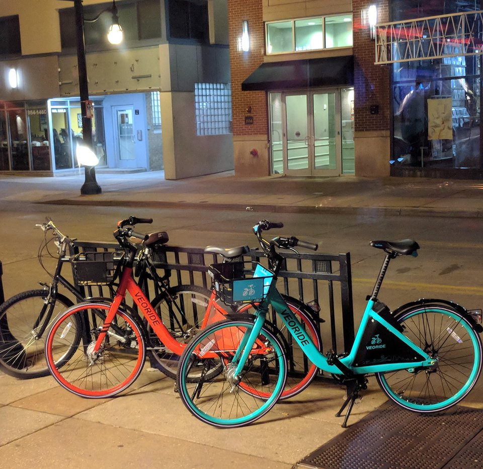
A key task in building AI systems is classification, e.g. identifying what's in a picture. For example, we might want to label each of the bikes in the above picture as either a veoride rental bike or a privately-owned bike. We'll start by looking at statistical methods of classification, particularly Naive Bayes.
Here are two types of ivy common in the northeastern US:
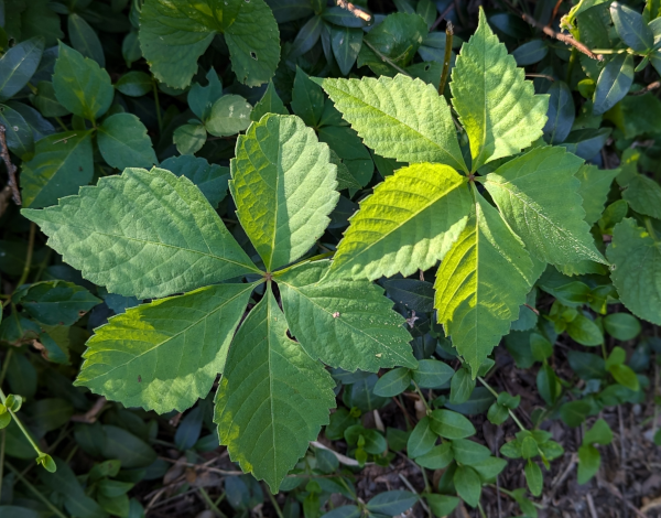
Five-finger ivy on the left and poison ivy on the right.
Poison ivy causes an itchy rash, so it's obviously important to be able to tell it from other types of ivy. The exact color isn't a reliable cue because it varies a lot even within the same species. The texture on the leaf margins is a bit different. But the cue that children are taught to use is that poison ivy has three leaflets in each cluster. (A completely accurate test also requires checking some other features such as whether it has thorns.)
Here are two CS faculty members. How would you describe the difference between Eric Shaffer and Paris Smaragdis in a way that would allow someone else to tell them apart, remembering that the color of their shirts isn't stable over time? A number of their obvious discrete features are the same: male, somewhat gray hair, smiling, light skin. Examples like this are where we need to use statistical or neural classification models, because they are better able to squeeze a classification from a set of real-valued features.
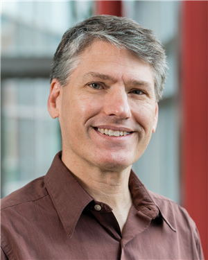
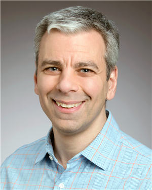
Eric Shaffer (left) and Paris Smaragdis (right) look similar in these pictures.
We can use discrete, logic-like features on simple situations. E.g. poison ivy has three leaflets in each group. However, our two faculty members share many easily-articulated features, e.g. both have gray hair. This style of model was popular through the 1980's, spawning long-lived projects to write rule sets that would let you distinguish (say) a potato from a sweet potato. But discrete features don't generalize well to many real-world situations. They are
In practice, this means that models based on yes/no answers to discrete features are incomplete and fragile There are many corner cases to consider, e.g. birds are supposedly defined partly by the fact that they lay eggs, but it's actually only the females who do that. Depending heavily on experts to craft, or even correct, rules only works well in domains like medicine, where there can be a large payoff for getting answers exactly right.
A better approach is to learn models from examples, e.g. pictures, audio data, big text collections. However, this input data presents a number of challenges:
So we use probabilistic models to capture what we know, and how well we know it.
Probabilities can be estimated from direct observation of examples (e.g. large corpus of text or labelled image data). Constraints on probabilities may also come from scientific beliefs:
The assumption that anything is possible is usually made to deal with the fact that our training data is incomplete, so we need to reserve some probability for all the possible events that we haven't happened to see yet. For example, I've never actually seen a raccoon in an engineering building, but it could happen. Maybe a zombie could even walk through the classroom door? Given some very small probability to unseen events also makes the system better able to handle mangled inputs, e.g. a sentence of text with a word left out.
Red and teal veoride bikes from
/u/civicsquid reddit post
Back to our bicycle example. We have two types of bike on our campus: Veoride rentals and privately owned bikes. Veorides are mostly teal (with a few exceptions), but other (privately owned) bikes are usually other colors. When the veorides were new, it became clear that teal isn't a popular color.
Here's the joint distribution for these two variables (numbers are guesswork):
                 veoride        private      |
    teal            0.19          0.02       |   0.21
    red             0.01          0.78       |   0.79
                 ----------------------------
                    0.20          0.80
For this toy example, we can fill out the full joint distribution table directly from observations, but that approach doesn't scale to more complex situations.
To develop suitable classification methods, we'll need to use Bayes Rule. Remember that P(A | C) is the probability of A in a context where C is true. For example, the probability of a bike being teal increases dramatically if we happen to know that it's a veobike.
P(teal) = 0.21
P(teal | veoride) = 0.95 (19/20)
The formal definition:of conditional probability is
P(A | C) = P(A,C)/P(C)
To derive Bayes Rule from this definition, let's write this in the equivalent form P(A,C) = P(C) * P(A | C).
We may have secret expectations for what A and C represent, but they are both just real numbers to the algebra. So we can flip the roles of A and C to get:
equivalently P(C,A) = P(A) * P(C | A)
P(A,C) and P(C,A) are the same quantity. (AND is commutative.) So we have
P(A) * P(C | A) = P(A,C) = P(C) * P(A | C)
So
P(A) * P(C | A) = P(C) * P(A | C)
So we have Bayes rule
P(C | A) = P(A | C) * P(C) / P(A)
Here's how to think about the pieces of this formula
       P(cause | evidence) =  P(evidence | cause) *  P(cause) / P(evidence)

         posterior            likelihood             prior     normalization
The normalization doesn't have a proper name because we'll typically organize our computation so as to eliminate it. Or, sometimes, we won't be able to measure it directly, so the number will be set at whatever is required to make all the probability values add up to 1.
Example: we see a teal bike. What is the chance that it's a veoride? We know
P(teal | veoride) = 0.95 [likelihood]
P(veoride) = 0.20 [prior]
P(teal) = 0.21 [normalization]
So we can calculate
P(veoride | teal) = 0.95 x 0.2 / 0.21 = 0.19/0.21 = 0.905
In non-toy examples, it will be easier to get estimates for P(evidence | cause) than direct estimates for P(cause | evidence).
P(evidence | cause) tends to be stable, because it is due to some underlying mechanism. In this example, veoride likes teal and regular bike owners don't. In a disease scenario, we might be looking at the tendency of measles to cause spots, which is due to a property of the virus that is fairly stable over time.
P(cause | evidence) is less stable, because it depends on the set of possible causes and how common they are right now.
For example, suppose that a critical brake problem is discovered and Veoride suddenly has to pull bikes into the shop for repairs. So then only 2% of the bikes are veorides. Then we might have the following joint distribution. Now a teal bike is more likely to be private rather than veoride.
                 veoride        private      |
    teal            0.019          0.025     |   0.044
    red             0.001          0.955     |   0.956
                 ----------------------------
                    0.02           0.98
Dividing P(cause | evidence) into P(evidence | cause) and P(cause) allows us to easily adjust for changes in P(cause).
Recall Bayes Rule:
       P(cause | evidence) =  P(evidence | cause) *  P(cause) / P(evidence)

       posterior            likelihood             prior     normalization
Example: We have two underlying types of bikes: veoride and private. We observe a teal bike. What type should we guess that it is?
"Maximum a posteriori" (MAP) estimate chooses the type with the highest posterior probability:
pick the type X such that P(X | evidence) is highest
Suppose that type X comes from a set of types T. Then MAP chooses
\(\arg\!\max_{X \in T} P(X | \text{evidence}) \)
The argmax operator iterates through a series of values for the dummy variable (X in this case). When it determines the maximum value for the quantity (P(X | evidence) in this example), it returns the value for X that produced that maximum value.
Completing our example, we compute two posterior probabilities:
P(veoride | teal) = 0.905
P(private | teal) = 0.095
The first probability is bigger, so we guess that it's a veoride. Notice that these two numbers add up to 1, as probabilities should.
P(evidence) can usually be factored out of these equations, because we are only trying to determine the relative probabilities. For the MAP estimate, in fact, we are only trying to find the largest probability. In our equation
P(cause | evidence) = P(evidence | cause) * P(cause) / P(evidence)
P(evidence) is the same for all the causes we are considering. Said another way, P(evidence) is the probability that we would see this evidence if we did a lot of observations. But our current situation is that we've actually seen this particular evidence and we don't really care if we're analyzing a common or unusual situation.
So Bayesian estimation often works with the equation
P(cause | evidence) \( \propto \) P(evidence | cause) * P(cause)
where we know (but may not always say) that the normalizing constant is the same across various such quantities.
Specifically, for our example
P(veoride | teal) = P(teal | veoride) * P(veoride) / P(teal)
P(private | teal) = P(teal | private) * P(private) / P(teal)
P(teal) is the same in both quantities. So we can remove it, giving us
P(veoride | teal) \( \propto \) P(teal | veoride) * P(veoride) = 0.95 * 0.2 = 0.19
P(private | teal) \( \propto \) P(teal | private) * P(private) = 0.025 * 0.8 = 0.02
So veoride is the MAP choice, and we never needed to know P(teal). Notice that the two numbers (0.19 and 0.02) don't add up to 1. So they aren't probabilities, even though their ratio is the ratio of the probabilities we're interested in.
As we saw above, our joint probabilities depend on the relative frequencies of the two underlying causes/types. Our MAP estimate reflects this by including the prior probability.
If we know that all causes are equally likely, we can set all P(cause) to the same value for all causes. In that case, we have
P(cause | evidence) \( \propto \) P(evidence | cause)
So we can pick the cause that maximizes P(evidence | cause). This is called the "Maximum Likelihood Estimate" (MLE).
The MLE estimate can be a sensible choice if we have poor information about the prior probabilities. But can also be very inaccurate if the prior probabilities of different causes are very different from one another. So if we have some approximate information about the prior, it's probably better to use that estimate in the MAP rather than resorting to the MLE.
The importance of the prior is often taught to medical students using the analogy of horses and zebras. If you hear hoofbeats in Urbana, you should guess that it's a horse, because horses are much more common than zebras around here. Medical students spend a lot of time memorizing details of rare diseases. So they tend to focus on those as candidates. But if they see a symptom like a rash, their first guess should be something common such as sunburn.
Red and teal veoride bikes from
/u/civicsquid reddit post
Suppose we are building a more complete bike recognition system. It might observe (e.g. with its camera) features like:
So our classification alogorithm looks like:
Input: a collection of objects of several types
Extract features from each object
Output: Use the features to label each object with its correct type
For example, we might wish to take a collection of documents (i.e. text files) and classify each document by type. For example:
Let's look at the British vs. American classification task. Certain words are characteristic of one dialect or the other. For example
The word "boffin" differs from "egghead" because it can be modified to make a wide range of derived words like "boffinry" and "astroboffin". Dialects have special words for local foods, e.g. the South African English words "biltong," "walkie-talkies," "bunny chow."
Bag of words model: We can use the individual words as features.
A bag of words model determines the class of a document based on how frequently each individual word occurs. It ignores the order in which words occur, which ones occur together, etc. So it will miss some details, e.g. the difference between "poisonous" and "not poisonous,"
How do we combine these types of evidence into one decision about whether the bike is a veoride?
However, when we have more features (typical of AI problems), this isn't practical. Suppose that each feature has two possible values. Then, if we observe the values of n features, we have \(2^n\) combinations of feature values. Each combination needs its own probability in the joint distribution table.
The estimation is the more important problem because we usually have only limited amounts of data, esp. clean annotated data. Many value combinations won't be observed simply because we haven't seen enough examples.
The Naive Bayes algorithm reduces the number of parameters to O(n) by making assumptions about how the variables interact,
Remember that two events A and B are independent iff
P(A,B) = P(A) * P(B)
Sadly, independence rarely holds. A more useful notion is conditional independence. That is, are two variables independent when we're in some limited context. Formally, two events A and B are conditionally independent given event C if and only if
P(A, B | C) = P(A|C) * P(B|C)
Conditional independence is also unlikely to hold exactly, but it is a sensible approximation in many modelling problems. For example, having a music stand is highly correlated with owning a violin. However, we may be able to treat the two as independent (without too much modelling error) in the context where the owner is known to be a musician.
The definiton of conditional independence is equivalent to either of the following equations:
P(A | B,C) = P(A | C)
P(B | A,C) = P(B | C)
It's a useful exercise to prove that this is true, because it will help you become familiar with the definitions and notation.
Suppose we're observing two types of evidence A and B related to cause C. So we have
P(C | A,B) \( \propto \) P(A,B | C) * P(C)
Suppose that A and B are conditionally independent given C. Then
P(A, B | C) = P(A|C) * P(B|C)
Substituting, we get
P(C | A,B) \( \propto \) P(A|C) * P(B|C) * P(C)
This model generalizes in the obvious way when we have more than two types of evidence to observe. Suppose our cause C has n types of evidence, i.e. random variables \( E_1,...,E_n \). Then we have
\( P(C | E_1,...E_n) \ \propto\ P(E_1|C) * ....* P(E_n|C) * P(C) \ = \ P(C) * \prod_{k=1}^n P(E_k|C) \)
So we can estimate the relationship to the cause separately for each type of evidence, then combine these pieces of information to get our MAP estimate. This means we don't have to estimate (i.e. from observational data) as many numbers. For n variables, each with two possible values (e.g. red vs teal), a naive Bayes model has only O(n) parameters to estimate, whereas the full joint distribution has \(2^n\) parameters.
Consider this sentence
The big cat saw the small cat.
It contains two pairs of repeated words. For example, \(W_3\) is "cat" and \(W_7\) is also "cat". Our estimation process will consider the two copies of "cat" separately
Jargon:
So our example sentence has seven tokens drawn from five types.
Depending on the specific types of text, it may be useful to normalize the words. For example
Stemming converts inflected forms of a word to a single standardized form. It removes prefixes and suffixes, leaving only the content part of the word (its "stem"). For example
       help, helping, helpful --->  help
       happy, happiness --> happi
Output is not always an actual word.
Stemmers are surprisingly old technology.
Porter made modest revisions to his stemmer over the years. But the version found in nltk (a currently popular natural language toolkit) is still very similar to the original 1980 algorithm.
Suppose that cause C produces n observable effects \( E_1,...,E_n \). Then our Naive Bayes model calculates the MAP estimate as
\( P(C | E_1,...E_n) \ \ \propto\ \ P(E_1|C) * ....* P(E_n|C) * P(C) \)
Rewriting slightly:
\( P(C | E_1,...E_n) \ \ \propto\ \ P(C) * \prod_{k=1}^n P(E_k|C) \)
Let's map this idea over to our Bag of Words model of text classification. Suppose our input document contains the string of words \( W_1, ..., W_n \). So \(W_k\) is the word token at position k. Suppose that \(P(W_k)\) is the probability of the corresponding word type.
To classify the document, naive Bayes compares these two values
\(P(\text{UK} | W_1, \ldots, W_n) \ \ \ \propto\ \ \ P(\text{UK}) \ * \ \prod_{k=1}^n P(W_k | \text{UK} ) \)
\( P(\text{US} | W_1, \ldots, W_n) \ \ \ \propto\ \ \ P(\text{US}) \ * \ \prod_{k=1}^n P(W_k | \text{US})\)
To do this, we need to estimate two types of parameters
Naive Bayes works quite well in practice, especially when coupled with a number of tricks that we'll see later. The conditional independence assumption is accurate enough for many applications and means that we have relatively few parameters to estimate from training data. The Naive Bayes spam classifier SpamCop, by Patrick Pantel and Dekang Lin (1998) got down to a 4.33% error rate using bigrams and some other tweaks.
A Quantitative Analysis of Lexical Differences Between Genders in Telephone Conversations Constantinos Boulis and Mari Ostendorf, ACL 2005
Fisher corpus of more than 16,000 transcribed telephone conversations (about 10 minutes each). Speakers were told what subject to discuss. Can we determine gender of the speaker from what words they used?
Words most useful for discriminating speaker's gender (i.e. used much more by men than women or vice versa)
This paper compares the accuracy of Naive Bayes to that of an SVM classifier, which is a more sophisticated classification technique.
The more sophisticated classifier makes an improvement, but not a dramatic one.
Training data: estimate the probability values we need for Naive Bayes
Development data: tuning algorithm details and high-level parameters
Test data: final evaluation (not always available to developer) or the data seen only when system is deployed
Training data only contains a sampling of possible inputs, hopefully typical inputs but nowhere near exhaustive. So development and test data will contain items that weren't in the training data. E.g. the training data might focus on apples where the development data has more discussion of oranges. Development data is used to make sure the system isn't too sensitive to these differences. The developer typically tests the algorithm both on the training data (where it should do well) and the development data. The final test is on the test data.
Now, let's look at estimating the probabilities. Suppose that we have a set of documents from a particular class C (e.g. English) and suppose that W is a word type. We can define:
count(W) = number of times W occurs in the documents
n = number of total words in the documents
A naive estimate of P(W|C) would be \(P(W | \text{C}) = \frac{\text{count}(W)}{n}\). This is not a stupid estimate, but a few adjustments will make it more accurate.
The probability of most words is very small. For example, the word "Markov" is uncommon outside technical discussions. (It was mistranscribed as "mark off" in the original Switchboard corpus.) Worse, our estimate for P(W|C) is the product of many small numbers. Our estimation process can produce numbers too small for standard floating point storage.
To avoid numerical problems, researchers typically convert all probabilities to logs. That is, our naive Bayes algorithm will be maximizing
\(\log(P(\text{C} | W_1,\ldots W_k))\ \ \propto \ \ \log(P(\text{C})) + \sum_{k=1}^n \log(P(W_k | \text{C}) ) \)
Notice that when we do the log transform, we need to replace multiplication with addition.
Recall that we train on one set of data, use the development data to tune parameters and algorithm design, and finally test on a different set of data. For example, in the Boulis and Ostendorf gender classifcation experiment, there were about 14M words of training/development data and about 3M words of test data. We usually hope that the training data are generally similar to the test data, but they won't be exactly the same. This is particularly true when the algorithm is tested by deploying it into some real application. The training and development data may have been collected in 2000-2024 but the final product is now running on inputs from 2025.
Training data doesn't contain all words of English and is too small to get a representative sampling of the words it contains. So for uncommon words:
Zeroes destroy the Naive Bayes algorithm. Suppose there is a zero on each side of the comparison. Then we're comparing zero to zero, although the other numbers may give us considerable information about the merits of the two outputs. We use "smoothing" algorithms to assign non-zero probabiities to unseen words.
Laplace smoothing is a simple technique for addressing the problem: In this method all unseen words are represented by a single word UNK. So the probability of UNK should represent all of these words collectively. Notice that P(UNK) is the probability of seeing one of this group of rare words. Each individual unseen word type has a low probability of appearing in the test data. However, since there are a very large number of rare word types, there is a significant chance that we'll see one of them.
n = number of words in our Class C training data
count(W) = number of times W appeared in Class C training data
To add some probability mass to UNK, we increase all of our estimates by \( \alpha \), where \(\alpha\) is a positive tuning constant, usually (but not always) no larger than 1. So our probabilities for UNK and for some other word W are:
P(UNK | C) = \(\alpha \over n\)
P(W | C) = \({count(W) + \alpha} \over n\)
This isn't quite right. Probabilities must add up to 1 and these numbers add up to \( n + \alpha(V+1) \) where V = number of word types seen in training data So we revise the denominators to make this be the case. Our final estimates of the probabilities are
V = number of word TYPES seen in training data
P(UNK | C) = \( \frac {\alpha}{ n + \alpha(V+1)} \)
P(W | C) = \( \frac {\text{count}(W) + \alpha}{ n + \alpha(V+1)} \)
When implementing Naive Bayes, notice that smoothing should be done separately for each class of document. For example, suppose you are classifying documents as UK vs. US English. Then Laplace smoothing for the UK English n and V would be the number of word tokens and word types seen in UK training data.