Natural language data (text, speech) is usually one-dimensional and has an inherent temporal ordering. Other types of data sometimes have similar structure, e.g. output from medical devices or industrial monitoring systems. This linear structure affects the typical choices for neural net architecture, in much the same way that the 2D structure of pictures causes CNNs to be an especially helpful design element. We'll concentrate on text examples because they are easier to explain.
Many sequential tasks fall into three types. We may be translating one sequence into another sequence (perhaps the same length, perhaps slightly different). For example:
In other cases, we are trying to provide a summary description for an extended piece of text. For example, we might want to classify a document as a CS lecture versus a newspaper article.
Finally, we may wish to digest a piece of input text and produce text of a very different form. For example
The input to a text processing system is typically a sequence of words. However, the number of words that a system *might* encounter is very large, if it is run on unrestricted text (e.g. scraped off the internet). So longer or less common input words are typically broken down into subword units by a tokenizer. This allows any English text input to be represented with a vocabulary of (say) 30,000 subwords. Popular tokenizers such as BPE (byte-pair encoding) and WordPiece rely primarily on compression-type criteria rather than linguistic structure (prefixes and suffixes).
WARNING: figures and examples in papers and tutorials typically continue to write the input using words, because that's easier to understand. And writers occasionally slip into using "word" when they probably mean "token".
To feed the token sequence into the first stage of our neural net, we convert each token into a vector using an embedding algorithm such as word2vec. Recall that these embedding vectors are relatively short and capture similarities in meaning between different words/tokens.
Some of the neural net processing steps preserve linear order. Others (notably transformers) tend to treat the input as a structureless bag of words. When this is a worry, the token embedding vectors are combined with a "positional encoding" vector which represents position in the input string in a way that subsequent neural processing can understand. The actual methods are more complex, but you can imagine a positional encoding vector as looking like a binary representation of the input position index.
You might be wondering how to combine two vectors, such as a word embedding and a positional encoding. This varies, depending on where we're doing it and sometimes with the design of a specific system. I'll let you look at the details in Jurafsky and Martin. There's three basic methods:
A similar (perhaps identical) vocabulary of tokens will be used when output text is generated. At each output position, last layer of the neural net produces a vector containing a probabilty for each token in the vocabulary. Softmax is usually used to normalize the amplitudes. Once a token is chosen for each output position, the sequence of tokens is translated back into a sequence of words.
Recurrent neural nets (RNNs) are neural nets that have connections that loop back from a layer to the same layer. The RNN shown below has a single hidden layer. We can think of the self-connected layer as containing multiple processing units, similar to the hidden layer of a normal neural network. The intent of the feedback loop in the picture is that each unit is connected to all the other units in the layer.
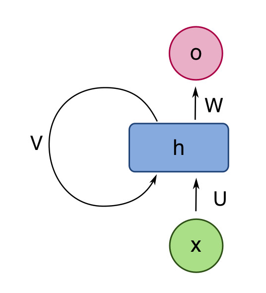 from Wikipedia
Alternatively, we can think of an RNN as a state machine. That is, we think of the values from all the units in the layer as bundled up into a state vector, \(s_i \) in the picture below. At each timestep, the RNN reads an input vector and the current state. It produces an output vector and a new state, using a state transition function (R), an output function (O), and some tunable parameters \(\theta\).
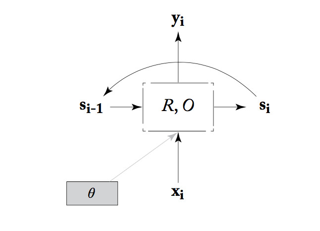 from Yoav Goldberg
To see how computation proceeds and, more importantly, how training works, we unroll the RNN. That is, we make a clone of the RNN for each timestep, creating the diagram below. Notice that all copies of the unit share the same parameter values.
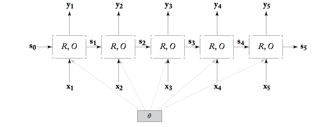 from Yoav Goldberg
An RNN can be used as a classifier. That is, the system using the RNN only cares about the output from the last timestep, as shown below. In an NLP system, the final output value may actually be complex, e.g. a summary of an entire sentence. Either way, the final output value is fed into a later processing that provides feedback about its performance (the loss value).
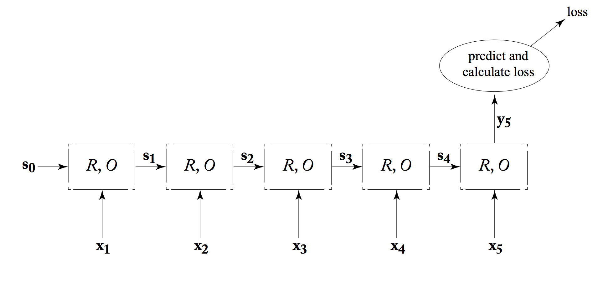 from Yoav Goldberg
This kind of RNN can be trained in much the same way as a standard ("feedforward") neural net. However, values and error signals propagate in the time direction. The forward pass calculates values moving to the right. Backpropagation starts at the final loss node and moves back to the left. This is often called "backpropagation through time." When the RNN is intended to operate on very long input sequences, they might need to be divided into shorter sections that are fed into the training process separately.
Like convolutional layers, RNNs rarely do an entire task by themselves. They are typically combined with other processing layers, either other types of neural net machinery or non-neural processing.
RNNs have proved most useful for modelling sequential data, which is common in natural language understanding and generation tasks. Some of these tasks use variations on the classifier design shown above. For example, many tasks require mapping the input sequence into a corresponding output sequence, e.g. mapping words to part-of-speech tags. In this case, we would care about getting the correct output at each timestep (not just the final one). So the connection to our loss function would look like this:
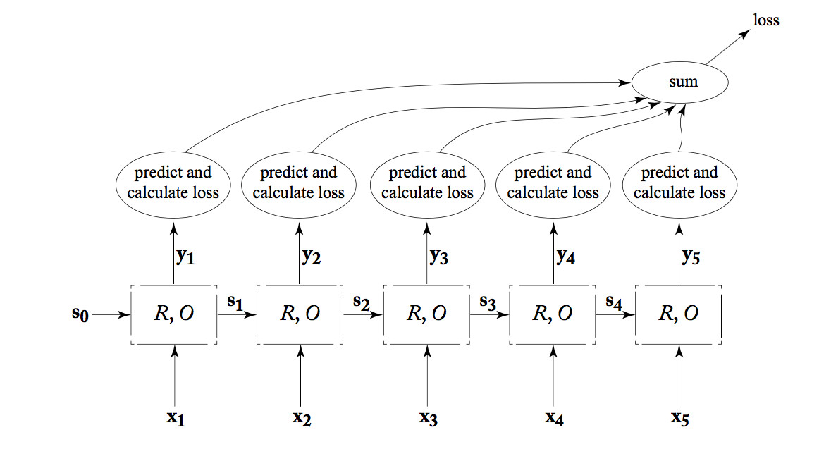 from Yoav Goldberg
We can join two RNN's together into a "bidirectional RNN." One RNN works forwards from the start of the input, the second works backwards from the end of the input. The output at each position is the concatenation of the two RNN outputs. This combined output would typically receive further processing (not shown) and then eventually be evaluated to produce a loss. When the loss information propagaes backwards, both RNNs receive feedback based on their joint answer.
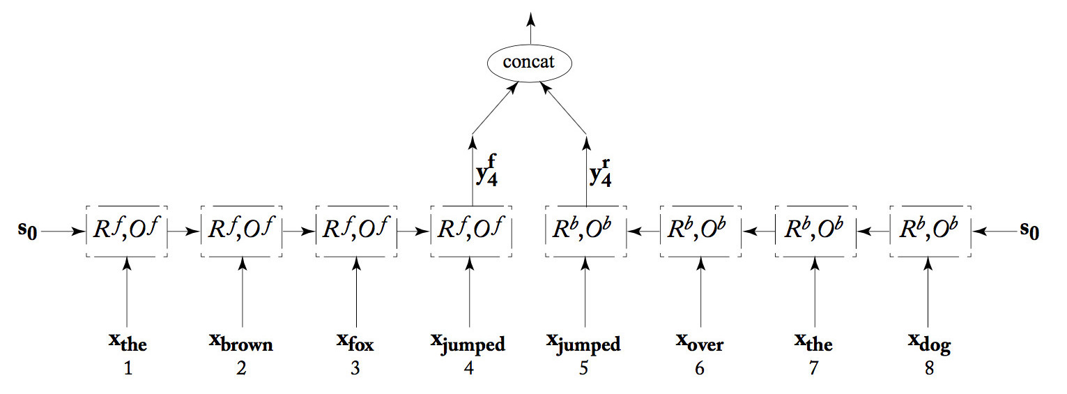 from Yoav Goldberg
We can also build "deep" RNN's, which have more than one processing layer between the input and output streams. The one shown below has three layers. Because each processing unit in an RNN is already complex (equivalent to multiple units in a standard neural net), it's unusual to see many layers.
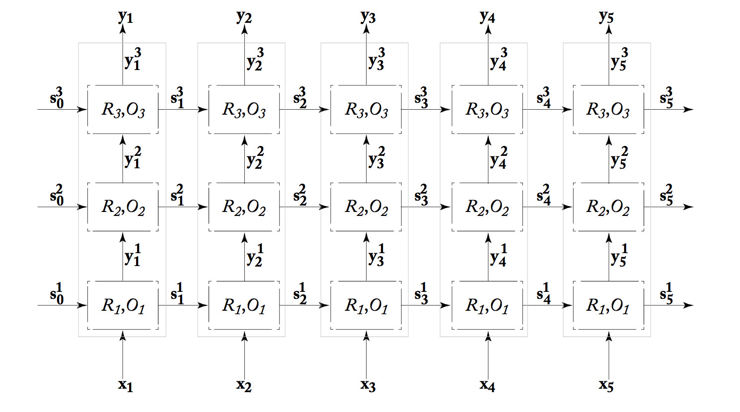 from Yoav Goldberg
In theory, an RNN can remember the entire stream of input values. However, gradient magnitude tends to decay as you move backwards from the loss signal. So earlier inputs may not contributed much to the RNN's final answer at the end. For a transducer, inputs may contribute little to the output for locations some distance away. This is a problem, because many linguistic tasks benefit from an extended context.
To allow RNNs to store information more effectively, researchers use "gated" versions of RNNs. These RNNs include separate vectors (the "gates") which control which parts of the unit's state will be updated at each timestep. The gates make the RNN's behavior easier to control, but create yet more tunable parameters that must be learned. Two popular gated RNN models are the "Long Short-Term Memory" (LSTM) and the "Gated Recurrent Unit" (GRU).
If we do a good job of managing the flow of information as the RNN reads the input sequence, then the RNN's hidden state after the final word of the input may be a good summary of the entire input. In that case, we can separate tasks such as translation into two components: an encoder that reads the input and a decoder that produces the output. The two are connected by a fixed-length context vector that summarizes everything that the decoder needs to know about the input. Encoder-decoder designs can be used for natural language translation, or for other tasks such as mapping text descriptions to/from pictures.

from Jurafsky and Martin
As we move through the input text, processing at each position (e.g. each input token) depends on the text that we've previously read. An HMM part of speech tagger makes its decisions based on the current word and the previous word, or previous couple words. The hidden state in an RNN contains a summary of the information at all previous positions. But, even with enhancements like LSTM, it's difficult to tune an RNN so that it remembers only the most relevant information and information from distant words is likely to be lost.
More recent sequential models keep a long buffer of previous tokens (e.g. like 1000 words) and use a technique called "attention" (or sometimes "self-attention") to extract appropriate information from these tokens. The short story is that we use a dot product to assess the similarity between each previous token and the token at our current processing position. This gives us a weight for each previous token. We then take a weighted average of the information from all previous tokens. This average summarizes the most relevant information from all the previous positions.
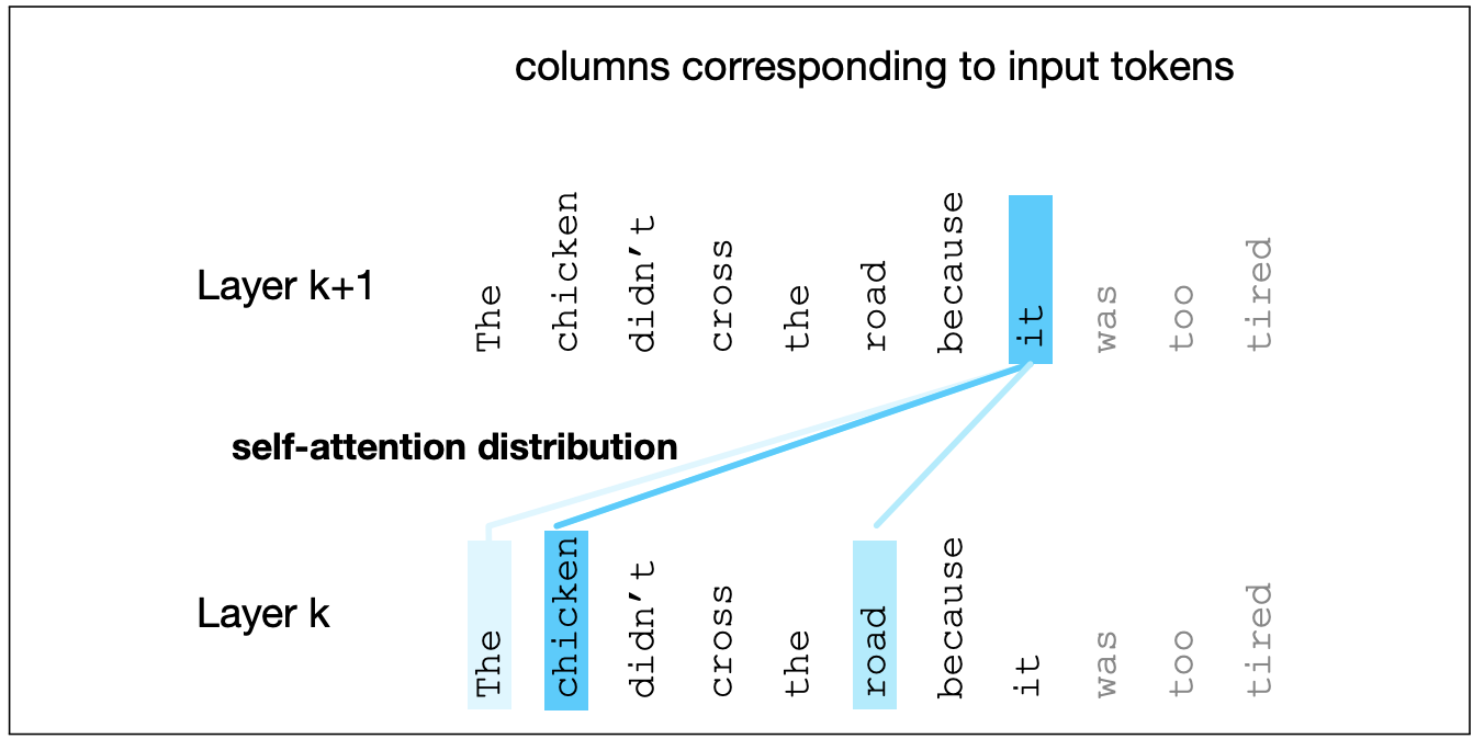 from Jurafsky and Martin
To make this work well, we don't actually use the raw token vectors in the weighted average computation. Rather, we convert the vector at our processing position into a "query" vector. The vector at each previous position is converted into a "key" vector and a "value" vector. These vectors are shorter than the original token vector and the conversions use sets of learned weights.
Once we have the query, key, and value vectors, the summary of information from previous positions is computed as follows:
This whole computational unit is called an "attention head".
In practice, modern networks typically set up multiple heads (e.g. perhaps 10 heads) that work in parallel. The algorithms for learning the conversion weights are randomized, so that each head learns a different set of weights and therefore (hopefully) learns to focus on a different aspect of the information in the previous text. Information from the heads is then combined before being given to later processing.
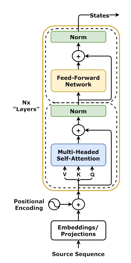
Attention is normally incorporated into a neural net architecture using "transformer blocks" Each transformer block contains an attention layer and a feed-forward neural network, plus some layers that normalize the values. Here are two examples:
from Wikipedia (Transformer article)
Notice that information flows through each of the two main sections (attention and the feed-forward network) but there are secondary paths that bypass each unit ("residual connections"). So the processed information is combined with a copy of the original input information.
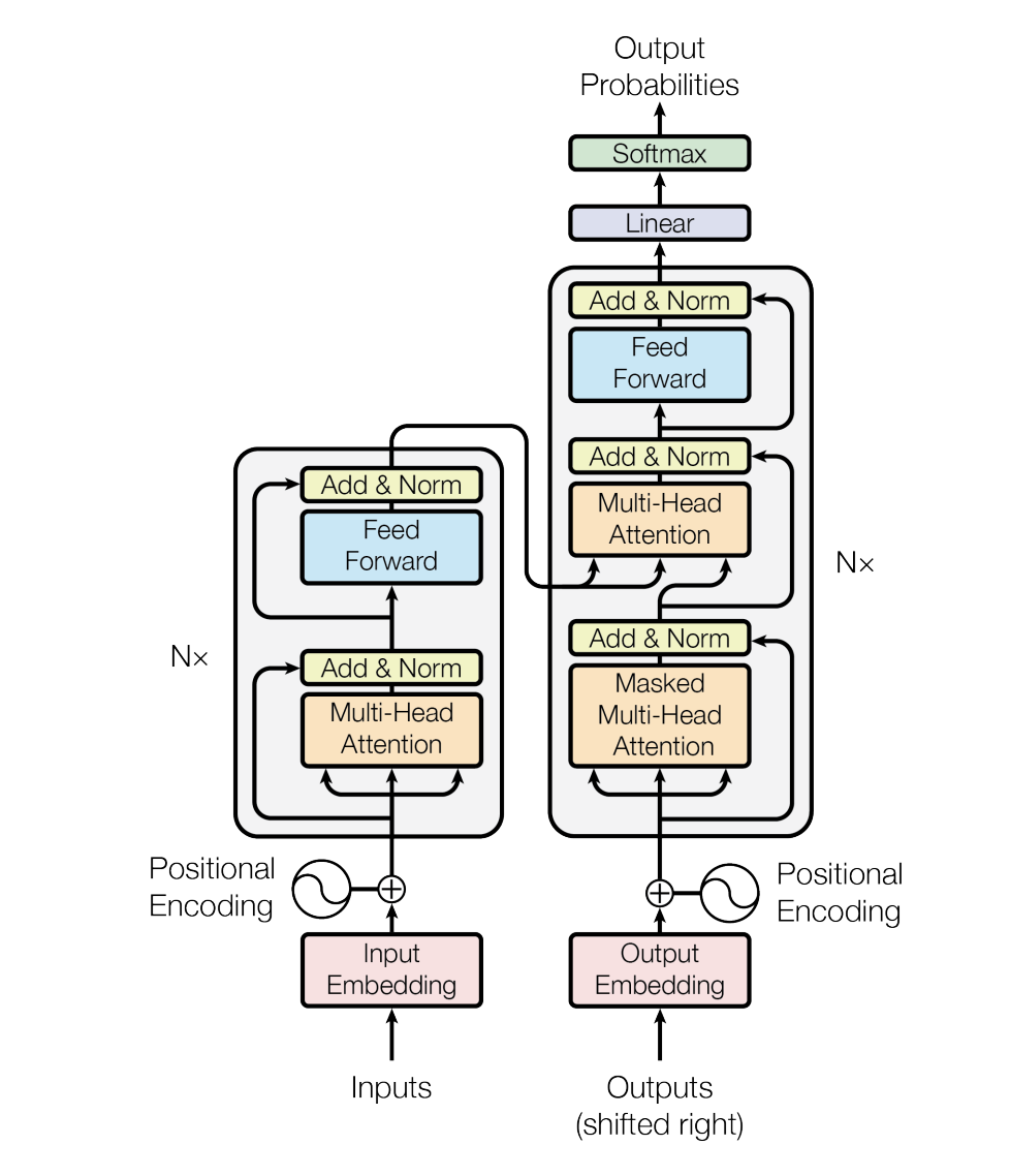
Historical note: transformers were introduced in a paper by a team from Google (Vaswani et al) in 2017. The attention mechanism was introduced slightly earlier, as an improvement to RNNs. Vaswani et al discovered that attention made it possible to avoid the recursive connections used in RNNs. The transformer design is complex but feed-forward.
Here is an example of a pair of transformer blocks in an encoder-decoder configuration. On the left is the encoder, a sequence of several transformers (6 in the original paper). These read in the input text and produce an output at the top. The output is fed into the decoder, a similar stack of transformers on the righthand side, which generate the output text. Because it is generating a sequence of words, not just one classification result, the input to the decoder also includes the text that it has generated so far, coming in from the bottom right in this figure.
from Vaswani et al 2017
The term "large language model" (LLM) is used to refer to two distinct typcs of design which appeared in close sequence: the first GPT model from OpenAI in 2018 and the BERT model from Google in 2019. Both make use of the transformer components sketched above. So-called "autogregressive" language models (e.g. the GPT family of models, the Llama family of models) read their input in order, with the attention mechanism drawing information only from words/tokens from the start through the current processing position. "Masked" language models (e.g. BERT) read the entire input in parallel, so the attention mechanism can draw information from words to either direction of a focus position. Both types are heavily used, because they are good for somewhat different purposes.
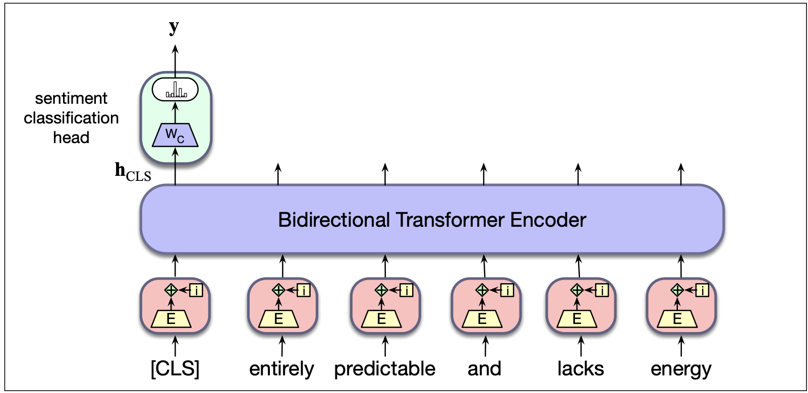
Configurations using these models often include the main bank of transformers and a "task head", as in the example below for BERT. The idea is that most of the training for the main part of the model is done on a large set of generic text and is suitable for generic tasks. The task head is then trained to use the model's output to accomplish some specific task (sentiment classification in this example), perhaps with some adjustment to the main model's weights. The first step is called "pre-training" and the second "fine-tuning".
from Jurafsky and Martin
Recent configurations of these models have often had very large sets of parameters and been training on astronomical amounts of data scraped off the web. So the initial pre-training process is very expensive and restricted to companies with large resources. Fine-tuning adjusts only a limited set of weights so that it can be done by people with more reasonable computing power.
Masked language models are primarily intended for classification tasks, such as deciding whether an input movie review is positive or negative. When properly tuned, the output layer provides context-dependent representations of the input words. For example, the word "bank" will be given output representations that are different in a financial context vs. a boating context.
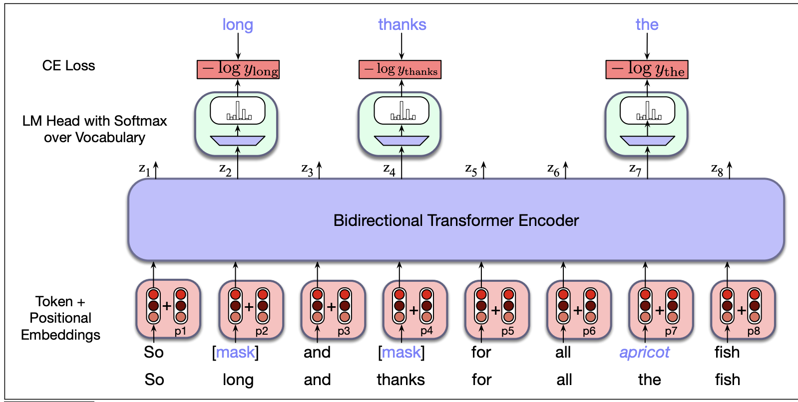
BERT is tuned using two tasks. In the first task, 15% of the input words are selected for possible corruption. At these positions, 80% of the words are replaced by "[MASK]", 10% are replaced with a random word, and 10% are left alone. The language model is trained to reconstruct the original words at these positions.
from Jurafsky and Martin
In the second training task, BERT is given two sentences as input, with separators at the start, end, and between the two sentences. The language model must decide whether the two sentences were adjacent in the training corpus or whether they were taken from different locations in the corpus. When sentences are adjacent, the second usually has a close relationship to the first, because text and spoken discourse are normally coherent.
After this pre-training, the final output (task head) can be adjusted for some similar language processing task, and then fine-tuned on that task.
The 2018 version of BERT had 340,000 parameters and was trained on a corpus of 3.3 billion words.
Autoregressive language models are primarily designed to generate text. The initial context for generation is provided by some amount of input text. Although they can be configured to do a range of different tasks, they are best known as a user interface that can answer a wide range of questions.
The main task for these models is predicting the next word, given a sequence of previous words. So the attention mechanism is looking at these previous words and the bank of transformers outputs its selection for the next word. (Well, ok, actually tokens rather than words ...) This training can be done by self-training: reading through large amounts of input text and trying, after each word, to predict the next one. At this level of abstraction, large language models are very similar to statistical language models that have been in use for decades (esp. in speech understanding).
What makes the recent generation of autoregressive models special is the length of the context used in doing this prediction. The context window for GPT-4 is 4096 tokens. For Llama-3, it's 8192 tokens. Training corpus sizes and batch sizes for weight adjustment are also insanely large and growing steadily. GPT-3 (2020) had 175 billion parameters and was trained on 300 billion words of text. This kind of training requires not only the right hardware, but significant amounts of power and (for cooling) water. Also, training data is limited by the amount on the internet, which is only expanding at a modest rate.
These context window sizes may seem huge. However, notice that 4096 tokens is less than 4096 words, and 4096 words is only about 10 pages of typewritten text. So this is enough to generate text that is very fluent, but it's not much context compared to the average length of a novel, which is perhaps 50,000 to 100,000 words. The weights in the neural net do also encode a fair amount of long-term information. But a recurring limitation of large language models is they lack the medium-term memory required to stay on topic or on task in extended conversations. They can start producing nonsense or repeating back memorized information if an attack manages to fill up their context window, e.g. asking ChatGPT to repeat a word thousands of times.
You might think that this problem could just be fixed by using even more training data to increase the length of the context window. That works somewhat. However, large language models are already hitting the limits of processing power and available training data. Also, there is a strong demand for language models small enough to be downloaded onto private machines or even small devices, such as toys. As this news story illustrates, processing on a central server is frequently unacceptable because both home users and business users want to keep their information private. Since the older generation of statistical language models were introduced in the 1980's, there has been a parallel line of research in how to compress language models by removing details likely to have a low impact on output quality.
Once the language model has been trained, generating text is relatively straightforward. The model starts with a context that comes from the user's prompt and predicts words one by one. As each new word is generated, it is added to the end of the context so that future words depend on the words that have already been generated. However, it doesn't work to simply pick the most likely word at each step, since most applications do not want the generator to say the exact same thing each time it encounters a given prompt. Rather, various randomization methods are used to select from the set of words that are most likely at each new position. (See Jurafsky and Martin, Chapter 10, for more details.)
The prompt given to the LLM is all important. LLMs can be fine-tuned by adjusting their weights (or the weights of a task head) using data from a specific domain. However, people often get them to do a specific task by describing the task in the prompt, perhaps including some concrete examples of correctly doing the task (input, output, justification or reasoning). Engineering suitable prompts has become a new area of research.
Two good references for further details are
These are the sources for figures above that are credited to those folks.