Since this class depends on data structures, which has discrete math as a prerequisite, most people have probably seen some version of BFS, DFS, and state graphs before. If this isn't true for you, this lecture probably went too fast. Aside from the textbook, you may wish to browse web pages for CS 173, CS 225, and/or web tutorials on BFS/DFS.
Key parts of a state graph:
Task: find a low-cost path from start state to a goal state.
Some applications want a minimum-cost path. Others may be ok with a path whose cost isn't stupidly bad (e.g. no loops).
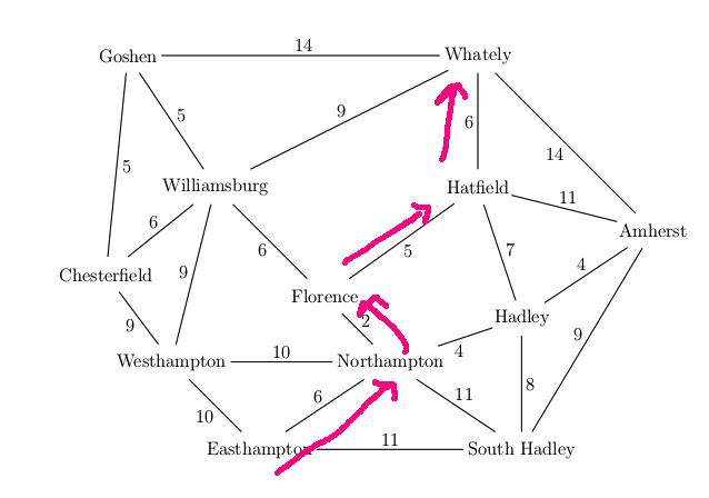
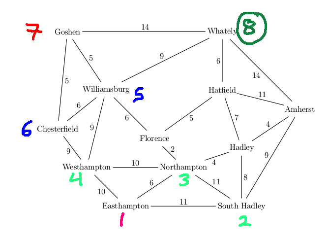
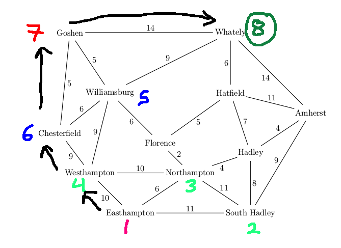
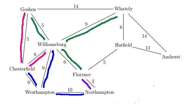
We can take a real-world map (below left) and turn it into a graph (below right). Notice that the graph is not even close to being a tree. So search algorithms have to actively prevent looping, e.g. by remember which locations they've already visited.
Mapping this onto a state graph:
On the graph, it's easy to see that there are many paths from
Northampton to Amherst, e.g. 8 miles via Hadley,
31 miles via Williamsburg and Whately.
Left below is an ASCII maze of the sort used in 1980's computer games.
R is the robot, G is the goal, F is a food pellet to collect
on the way to the goal. We no longer play games of this style,
but you can still find search problems with this kind of simple
structure. On the right is one path to the goal. Notice that
it has to double back on itself in two places.
Modelling this as a state graph:
Some mazes impose tight constraints on where the robot can go,
e.g. the bottom corridor in the above maze is only one cell wide.
Mazes with large open areas can have vast numbers of possible
solutions. For example, the maze below has many paths from start to
goal. In this case, the robot needs to move 10 steps right and 10
steps down. Since there are no walls constraining the order of right
vs. downward moves, there are \(20 \choose 10 \) paths of shortest
length (20 steps), which is about 185,000 paths.
We need to quickly choose one of these paths rather than wasting
time exploring all of them individually.
Game mazes also illustrate another feature that appears in some AI
problems: the AI gains access to the state graph as it explores.
E.g. at the start of the game, the map may actually look like this:
States may also be descriptins of the real world in terms of feature values.
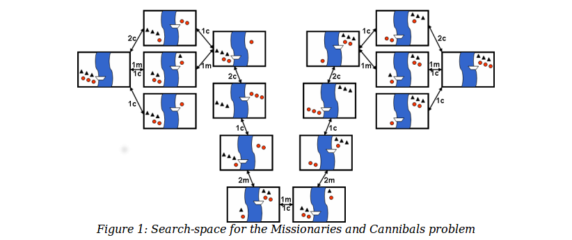
For example, consider the
Missionaries and Cannibals puzzle. In the starting state, there
are three missionaries, three cannibals, and a boat on the left side of a
river. We need to move all six people to the right side, subject to
the following constraints:
The state of the world can be described by three variables: how many missionaries on
the left bank, how many cannibals on the left bank, and which bank the boat is on.
The state space is shown below:
In this example
In speech recognition, we need to transcribe an acoustic waveform into
to produce written text. We'll see details of this process later in the
course. For now, just notice that this proceeds word-by-word.
So we have a set of candidate transcriptions for the first part of
the waveform and wish to extend those by one more word. For example,
one candidate transcription might start with "The book was very" and
the acoustic matcher says that the next word sounds like "short" or "sort."
In this example
Speech recognition systems have vast state spaces. A recognition
dictionary may know about 100,000 different words. Because acoustic
matching is still somewhat error-prone, there may be many words that
seem to match the next section of the input. So the
currently-relevant states are constructed on demand, as we search.
Chess is another example of an AI problem with a vast state space.
For all but the simplest AI problems, it's easy for a search algorithm to
get lost.
The first two of these can send the program into an infinite loop. The
third and fourth can cause it to get lost, exploring states
very far from a reasonable path from the start to the goal.
Our first few search algorithms will be uninformed. That is, they
rely only on computed distances from the starting state. Next week,
we'll see \(A^*\). It's an informed search algorithm because it
also uses an estimate of the distance remaining to reach the goal.
A state is exactly one of
Basic outline for search code
Data structure for frontier determines type of search
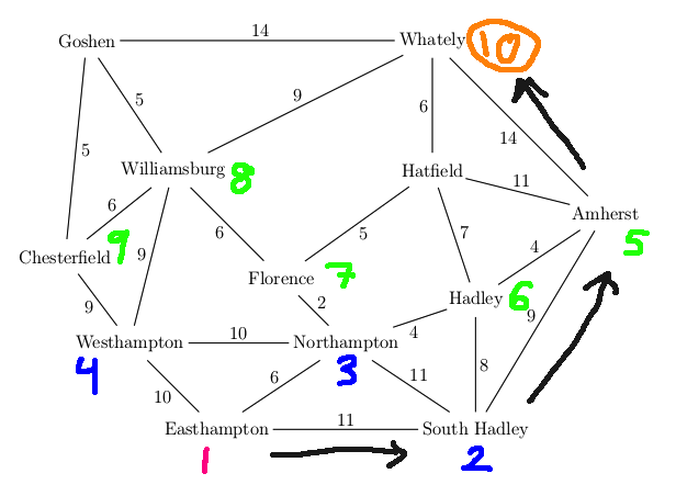
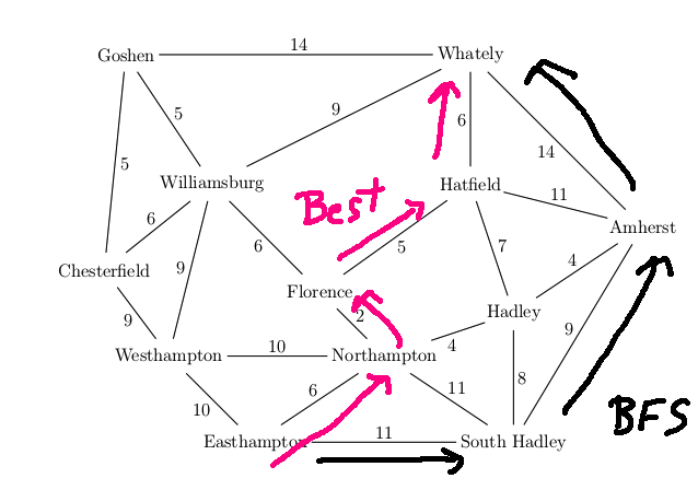
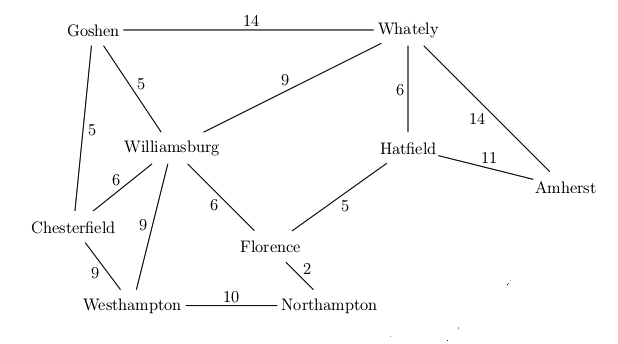
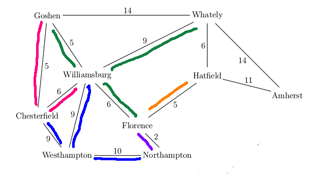
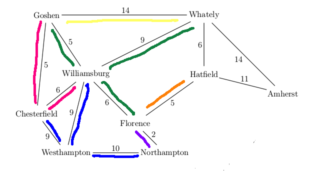
Let's find a route from Easthampton to Whately in our example map.
The actual best route is via Northampton, Florence, Hatfield (19 miles)
Suppose we use breadth-first search to find a route.
The frontier is stored as a queue. So we explore locations in
rings, gradually moving outwards from the starting location.
Let's assume we always explore edges counterclockwise (right to left).
A trace of the algorithm looks like this:
We return the path Easthampton, South Hadley, Amherst, Whately (length 34).
This isn't the shortest path
by mileage, but it's one of the shortest paths by number of edges.
BFS properties:
Here is a fun animation of
BFS set to music.
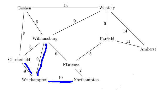
The frontier is stored as a stack (explicitly or implicitly via recursive function calls).
Again, we'll explore edges counterclockwise.
Detailed trace:
We return the path: Easthampton, Westhampton, Chesterfield, Goshen, Whately (length 38)
DFS properties:
If the search space is finite and you make sure the algorithm doesn't
loop back to already-seen states (see below), then DFS will find the
goal if it's reacheable. However, this isn't theoretically
true if the search space
is infinite, which is common in AI. In practice, an infinite search
space means that the search space is being built dynamically and
DFS may exhaust time or memory before finding the goal.
Animation of
DFS set to music.
Compare this to the one for BFS.
There are several basic tricks required to make DFS and BFS work right.
First, store the list of seen states, so that your code can tell when it has
returned to a state that has already been explored. Otherwise, your code may
end up in an infinite loop and/or be massively inefficient.
Second, return as soon as a goal state has been found. The entire space of states
may be infinite. Even when it is finite, searching the entire set of states is inefficient.
Third, don't use recursion to implement DFS unless paths are known to be short.
A small number of programming languages make this safe by optimizing tail recursion.
More commonly, each recursive call allocates stack space and you are likely to
exceed limits on stack size and/or recursion depth.
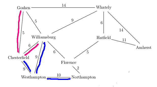
When a search algorithm finds the goal, it must be able to return best
path to the goal.
So, during search, each seen state must remember the best path back to the start state.
To do this efficiently, each state stores a
pointer to the previous state in the
best path, called a backpointer.
When the goal is found, we retrieve the best path by chaining backwards
using the backpointers until we reach the start state.
For example, suppose that our search algorithm has started from
Easthampton and has explored all the
blue edges in the map below. For each town, there is a best path
back to Easthampton using only the edges explored so far (blue edges).
For example, the best path for Williamsburg is via Westhampton.
We've also seen a route to Williamsburg via Chesterfield and another
via Goshen, but these are both
longer. So the backpointer for Williamsburg (in red) goes to Westhampton.
When we've seen two routes of the same length, you can pick either
when storing the backpointer.
We can dramatically improve the low-memory version of DFS by
running it with a progressively increasing bound on the maximum path
length. This is a bit like having a dog running around you on
a leash, and gradually letting the leash out.
Specifically:
This is called "iterative deepening." Its properties
Each iteration repeats the work of the previous one.
So iterative
deepening is most useful when the new search area at distance k is large
compared to the area search in previous iterations, so that the search
at distance k is dominated by the paths of length k.
These conditions don't hold for 2D mazes. The search area at radius k
is proportional to k, whereas the area inside that radius is proportional
to \(k^2\).
However, suppose that the search space looks like a 4-ary tree. We know from
discrete math that there are \(4^k\) nodes at level k. Using a geometric
series, we find that there are \(1/3\cdot (4^k -1)\) nodes in levels 1 through k-1.
So the nodes in the lowest level dominate the search. This type of
situation holds (approximately) for big games such as chess.
Backwards and bidirectional search are
basically what they sound like. Backwards search is like forwards search
except that you start from the goal. In bidirectional search, you
run two parallel searches, starting from start
and goal states, in hopes that they will connect at a shared state.
These approaches are useful only in very specific situations.
Backwards search makes sense
when you have relatively few goal states, known at the start.
This often fails, e.g. chess has a huge number of winning board configurations.
Also, actions must be easy to run backwards (often true).
Example: James Bond is driving his Lexus in central Boston and wants to get
to Dr. Evil's lair in Hawley, MA (population 337). There's a vast
number of ways to get out of Boston but only one road of significant
size going through Hawley. In that situation, working backwards from
the goal might be much better than working forwards from the starting
state.
Breadth-first search returns a path that uses the fewest edges.
However, this may not be the shortest path.
Breadth-first search only returns an optimal path if all edges
have the same cost (e.g. length).
In the example below, the shortest path has length 19 and the
BFS path has length 34.
Uniform-cost search (UCS) is a similar algorithm
that finds optimal paths even when edge costs vary.
Recall that the frontier in a search algorithm
contains states that have been seen
but their outgoing edges have not yet been explored. BFS stores the
frontier as a queue; DFS stores it as a stack.
Uniform-cost search stores the frontier as a priority queue.
So, in each iteration of our
UCS search loop, we
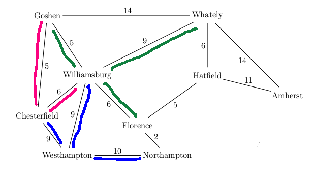
Want to find best route from Westhampton to Hatfield in this simplified map
A new feature in UCS search is that our first visit to a state may not be via the
best path to that state. E.g. we had to update the distance to Florence the
second time we visited it. It's usually best to keep a separate table of the
best distances (so far) to each state, so that we can quickly check whether a
distance needs to be updated.
When we update the distance to a state, we also need to update the backpointer to the
previous state along the new (better) route.
We also cannot stop the search right away when we reach a goal state.
We've found one route to the goal, but perhaps not the best one.
So we need to put the goal state back onto the frontier.
We stop the search when the goal state reaches the top of the priority queue, i.e.
when all states in the priority queue have a distance that is at least as large
as the goal state.
Efficient priority queue implementations (e.g. the ones supplied with your favorite programming
language) don't necessarily support updates to the priority numbers.
In many applications, decreases in state cost aren't very frequent. So this creates
less inefficiency than using a priority queue implementation with more features.
To do the analysis right, we need to assume
These assumptions are almost always true in practical uses of these
algorithms. If they aren't true, algorithm design and analysis can
get much harder in ways that are beyond the scope of this class.
Given those assumptions, UCS returns an optimal path even if edge costs vary.
Memory requirements for UCS are similar to BFS. They can be worse than BFS
in some cases, because UCS can get stuck in extended areas of short
edges rather than exploring longer but more promising edges.
You may have seen Dijkstra's algorithm in data structures class. It
is basically similar to UCS, except that it finds the distance from the
start to all states rather than stopping when it reaches a designated goal state.
Mazes
Puzzle
 (from
Gerhard Wickler, U. Edinburgh)
(from
Gerhard Wickler, U. Edinburgh)
Speech recognition
Some high-level points
Recap
Basic search outline
Loop until we find a solution
Map example
BFS
DFS
Basic tricks
Returning paths
Length-bounded DFS
DFS performs very poorly when applied directly to most search problems.
However, it becomes the method of choice when we have a tight bound on
the length of the solution path. This happens in two types of situations,
which we'll see later in the course:
In this situation, DFS can be implemented so as to use very little
memory. In AI problems, the set of seen states can often become
very large, so that programs can run out of memory or put enough
pressure on the system memory management that programs slow down.
Instead of storing and checking this large set, length-bounded DFS
checks only that the current path contains no duplicate states.
There is a tradeoff here. Checking only the current path will
cause the algorithm to re-do some of its search work, because it
can't remember what states has already searched. In practice, the
wisdom of this approach depends on the application.
When there are tight bounds on path length, it's safe to implement
DFS using recursion rather than a stack.
Iterative deepening
For k = 1 to infinity
Run DFS but stop whenever a path contains at least k states.
Halt when we find a goal state
Backwards and Bidirectional Search
Uniform-cost search
UCS Example
Some algorithm details for UCS
Workaround: it may be more efficient to put a second copy of the state (with the
new cost) into the priority queue.
Properties of UCS