Discrete random variables

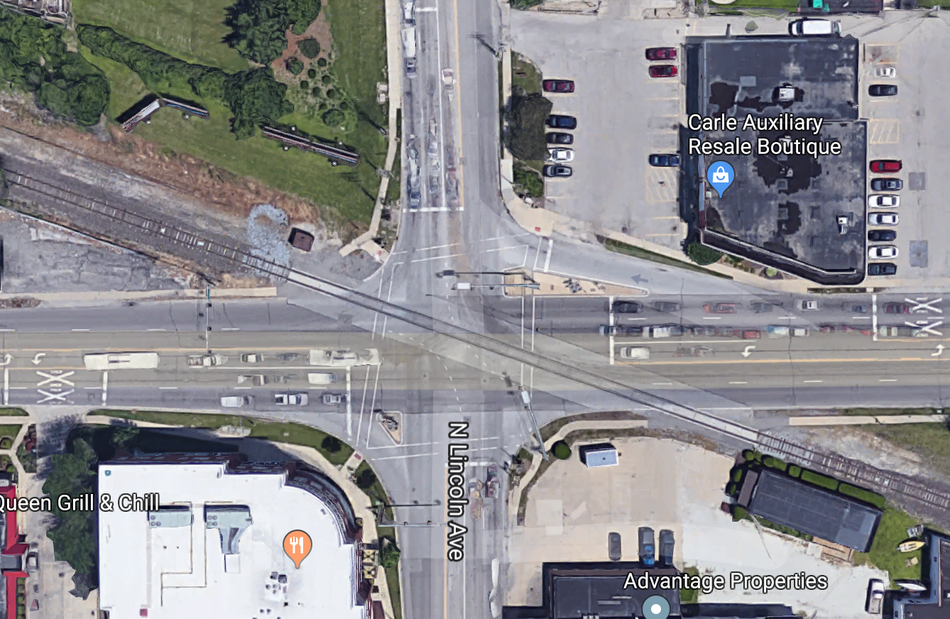
Suppose we're modelling the traffic light at University and Lincoln (two crossing streets plus a diagonal train track).

Some useful random variables might be:

Also exist continuous random variables, e.g. temperature (domain is all positive real numbers) or course-average (domain is [0-100]). We'll ignore those for now.

A state/event is represented by the values for all random variables that we care about.

Probabilities

P(variable = value) or P(A) where A is an event

What percentage of the time does [variable] occur with [value]? E.g. P(barrier-arm = up) = 0.95

P(X=v and Y=w) or P(X=v,Y=w)

How often do we see X=v and Y=w at the same time? E.g. P(barrier-arm=up, time=morning) would be the probability that we see a barrier arm in the up position in the morning.

P(v) or P(v,w)

The author hopes that the reader can guess what variables these values belong to. For example, in context, it may be obvious that P(up, morning) is shorthand for P(barrier-arm=up, time=morning).

Probability notation does a poor job of distinguishing variables and values. So it is very important to keep an eye on types of variable and values, as well as the general context of what an author is trying to say. A useful heuristic is that

• variables are usually capital letters, and
• values are usually lowercase letters.

A distribution is an assignment of probability values to all events of interest, e.g. all values for particular random variable or pair of random variables.

Properties of probabilities

The key mathematical properities of a probability distribution can be derived from Kolmogorov's axioms of probability:

0 \( \le \) P(A)

P(True) = 1

P(A or B) = P(A) + P(B), if A and B are mutually exclusive events

It's easy to expand these three axioms into a more complete set of basic rules, e.g.

0 \( \le \) P(A) \( \le \) 1

P(True) = 1 and P(False) = 0

P(A or B) = P(A) + P(B) - P(A and B) [inclusion/exclusion, same as set theory]

If X has possible values p,q,r, then P(X=p or X=q or X=r) = 1.

Joint probabilities

Here's a model of two variables for the Lincoln and University intersection (we're going to ignore the train track for simplicity):

                             E/W light                
                        green       yellow   red
 N/S light   green        0          0       0.2      
             yellow       0          0       0.1      
             red         0.5         0.1     0.1

To be a probability distribution, the numbers must add up to 1 (which they do in this example).

Most model-builders assume that probabilities aren't actually zero. That is, unobserved events do occur but they just happen so infrequently that we haven't yet observed one. So a more realistic model might be

                             E/W light              
                        green         yellow     red
 N/S light   green        e            e         0.2-f       
             yellow       e            e         0.1-f       
             red         0.5-f       0.1-f       0.1-f           

To make this a proper probability distribution, we need to set f=(4/5)e so all the values add up to 1.

Suppose we are given a joint distribution like the one above, but we want to pay attention to only one variable. To get its distribution, we sum probabilities across all values of the other variable.

                             E/W light                marginals
                        green       yellow   red
 N/S light   green        0          0       0.2        0.2
             yellow       0          0       0.1        0.1
             red         0.5         0.1     0.1        0.7
-------------------------------------------------
marginals                0.5         0.1     0.4

So the marginal distribution of the N/S light is

P(green) = 0.2
P(yellow) = 0.1
P(red) = 0.7

To write this in formal notation suppose Y has values \( y_1 ... y_n \). Then we compute the marginal probability P(X=x) using the formula \( P(X=x) = \sum_{k=1}^n P(x,y_k) \).

Conditional probabilities

Suppose we know that the N/S light is red, what are the probabilities for the E/W light? Let's just extract that line of our joint distribution.

                             E/W light               
                        green       yellow      red
 N/S light   red         0.5         0.1         0.1   

The notation for a conditional probability looks like P(event | context).

If we just pull numbers out of this row of our joint distribution, we get a distribution that looks like this:

P(E/W=green | N/S = red) = 0.5
P(E/W=yellow | N/S = red) = 0.1
P(E/W=red | N/S = red) = 0.1

Oops, these three probabilities don't sum to 1. So this isn't a legit probability distribution (see Kolmogorov's Axioms above). To make them sum to 1, divide each one by the sum they currently have (which is 0.7). So, in the context where N/S is red, we have this distribution:

P(E/W=green) = 0.5/0.7 = 5/7
P(E/W=yellow) = 0.1/0.7 = 1/7
P(E/W=red) = 0.1/0.7 = 1/7

Conditional probability equations

Conditional probability models how frequently we see each variable value in some context (e.g. how often is the barrier-arm down if it's nighttime). The conditional probability of A in a context C is defined to be

P(A | C) = P(A,C)/P(C)

Many other useful formulas can be derived from this definition plus the basic formulas given above. In particular, we can transform this definition into

P(A,C) = P(C) * P(A | C)
P(A,C) = P(A) * P(C | A)

These formulas extend to multiple inputs like this:

P(A,B,C) = P(A) * P(B | A) * P(C | A,B)

Independence

Two events A and B are independent iff

P(A,B) = P(A) * P(B)

It's equivalent to show that this equation is equivalent to each of the following equations:

P(A | B) = P(A)
P(B | A) = P(B)

Exercise for the reader: why are these three equations all equivalent? Hint: use definition of conditional probability. Figure this out for yourself, because it will help you become familiar with the definitions.

Metrics for Evaluating a Classifer

Results of classification experiments are often summarized into a few key numbers. There is often an implicit assumption that the problem is asymmetrical: one of the two classes (e.g. Cancer) is the target class that we're trying to identify.

We can summarize performance using the rates at which errors occur:

• False positive rate = FP/(FP+TN) [how many wrong things are in the negative outputs]
• False negative rate = FN/(TP+FN) [how many wrong things are in the positive outputs]
• Accuracy = (TP+TN)/(TP+TN+FP+FN)
• Error rate = 1-accuracy

Now, suppose we have a task that's well described as extracting a specific set of items from a larger input set. We can ask how well our output set contains all, and only, the desired items:

• precision (p) = TP/(TP+FP) [how many of our outputs were correct?]
• recall (r) = TP/(TP+FN) [how many of the correct answers did we find?]
• F1 = 2pr/(p+r)

F1 is the harmonic mean of precision and recall. Both recall and precision need to be good to get a high F1 value.

For more details, see the Wikipedia page on recall and precision

We can also display a confusion matrix, showing how often each class is mislabelled as a different class. These usually appear when there are more than two class labels. They are most informative when there is some type of normalization, either in the original test data or in constructing the table. So in the table below, each row sums to 100. This makes it easy to see that the algorithm is producing label A more often than it should, and label C less often.